Books / Introduction to C Programming Language / Chapter 32

Trees

Divide and conquer yields algorithms whose execution has a tree structure. Sometimes we build data structures that are also trees. It is probably not surprising that divide and conquer is the natural way to build algorithms that use such trees as inputs.

Tree basics

Here is a typical binary tree. It is binary because every node has at most two children; not all trees will have this property, but it is common for tree data structures that implement divide-and-conquer, because it yields simpler code.

This particular tree is also complete because the nodes consist only of internal nodes with exactly two children and leaves with no children. Not all binary trees will be complete.

Structurally, a complete binary tree consists of either a single node (a leaf) or a root node with a left and right subtree, each of which is itself either a leaf or a root node with two subtrees. The set of all nodes underneath a particular node x is called the subtree rooted at x.

A binary tree is a data structure that consists of a group of nodes organized in a specific hierarchy: each node in a binary tree has at most two children, which are named left child and the right child. The top-most node is called the root node. Nodes that don’t have any children are called leave nodes.

Binary trees are a popular data structure in computer science. One of the main advantages of binary trees is that they allow efficient insertion, deletion, and search operations in many situations. For example, you can use a binary tree to store a large number of items in a way that allows you to quickly find a specific item by its key.

Binary trees are also used in many other areas of computer science, including algorithm design, compiler design, and artificial intelligence.

The size of a tree is the number of nodes; a leaf by itself has size 1. The height of a tree is the length of the longest path; 0 for a leaf, at least one in any larger tree. The depth of a node is the length of the path from the root to that node. The height of a node is the height of the subtree of which it is the root, i.e. the length of the longest path from that node to some leaf below it. A node u is an ancestor of a node v if v is contained in the subtree rooted at u; we may write equivalently that v is a descendant of u. Note that every node is both an ancestor and a descendant of itself. If we wish to exclude the node itself, we refer to a proper ancestor or proper descendant.

Trees arise in programs in two ways:

Because we are dealing with tree-structured data. Family trees, HTML documents, parse trees — these are all examples of data that is already organized as a tree. In this case the data structure in the program reflects the structure of the data. Such trees are often not binary, since we don’t have control over how many children each node has. See Tree-structured data below.
Because we are dealing with tree data structures. These are data structures that are organized by splitting the data in half recursively. Examples are heaps and binary search trees.

We’ll start by talking about general trees and then concentrate mostly on binary trees.

Tree-structured data

Data from the outside world is often organized in trees. This is particularly true for code of various kinds.

For example, HTML explicitly encodes a tree, where each node in the tree is either a formatting tag or raw text. Formatting tags translate into internal nodes, and the contents between the opening and closing tag translate to the children of these nodes. For example, the short HTML file

<HTML>
    <HEAD>
        <TITLE>Title!</TITLE>
    </HEAD>
    <BODY>
        <P>This paragraph has <EM>emphasized text.</EM></P>
        <P>This paragraph has <B>bold.</B></P>
    </BODY>

turns into the tree

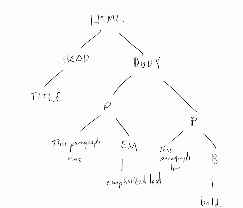
To represent a tree like this in C, we need a recursive data structure that includes enough information to identify the type and contents of each node, as well as pointers to all the children of each internal node. Something like this might work:

struct htmlNode {
    enum { TYPE_TAG, TYPE_TEXT } type;
    char *value;             // tag name or text contents
    struct htmlNode **kids;  // if non-null, null-terminated sequence of pointers
};

Similar parse tree data structures are often used in programming language compilers and interpreters to represent source code. This allows the compiler/interpreter to concentrate on the structure of the code instead of having to worry about unstructured sequences of characters. A simple example is given in .

Because of the complexity of handling arbitrary numbers of children, if we aren’t forced to do it, we will often instead use a binary tree, where each node has at most two children.

Binary trees

A binary tree typically looks like a linked list with an extra outgoing pointer from each element, as in

struct node {
    int key;
    struct node *left;  /* left child */
    struct node *right; /* right child */
};

An alternative is to put the pointers to the children in an array. This lets us loop over both children, pass in which child we are interested in to a function as an argument, or even change the number of children:

#define NUM_CHILDREN (2)

struct node {
    int key;
    struct node *child[NUM_CHILDREN];
};

Which approach we take is going to be a function of how much we like writing left and right vs child[0] and child[1]. A possible advantage of left and right is that it is harder to make mistakes that are not caught by the compiler (child[2]). Using the preprocessor, it is in principle possible to have your cake and eat it too (#define left child[0]), but I would not recommend this unless you are deliberately trying to confuse people.

Missing children (and the empty tree) are represented by null pointers. Typically, individual tree nodes are allocated separately using malloc; however, for high-performance use it is not unusual for tree libraries to do their own storage allocation out of large blocks obtained from malloc.

Optionally, the struct may be extended to include additional information such as a pointer to the node’s parent, hints for balancing, or aggregate information about the subtree rooted at the node such as its size or the sum/max/average of the keys of its nodes.

When it is not important to be able to move large subtrees around simply by adjusting pointers, a tree may be represented implicitly by packing it into an array. This is a standard approach for implementing heaps, which we will see soon.

The canonical binary tree algorithm

Pretty much every divide and conquer algorithm for binary trees looks like this:

void
doSomethingToAllNodes(struct node *root)
{
    if(root) {
        doSomethingTo(root);
        doSomethingToAllNodes(root->left);
        doSomethingToAllNodes(root->right);
    }
}

The function processes all nodes in what is called a preorder traversal, where the “preorder” part means that the root of any tree is processed first. Moving the call to doSomethingTo in between or after the two recursive calls yields an inorder or postorder traversal, respectively.

In practice we usually want to extract some information from the tree. For example, this function computes the size of a tree:

int
treeSize(struct node *root)
{
    if(root == 0) {
        return 0;
    } else {
        return 1 + treeSize(root->left) + treeSize(root->right);
    }
}

and this function computes the height:

int
treeHeight(struct node *root)
{
    int lh;     /* height of left subtree */
    int rh;     /* height of right subtree */

    if(root == 0) {
        return -1;
    } else {
        lh = treeHeight(root->left);
        rh = treeHeight(root->right);
        return 1 + (lh > rh ? lh : rh);
    }
}

Since both of these algorithms have the same structure, they both have the same asymptotic running time. We can compute this running time by observing that each recursive call to treeSize or treeHeight that does not get a null pointer passed to it gets a different node (so there are n such calls), and each call that does get a null pointer passed to it is called by a routine that doesn’t, and that there are at most two such calls per node. Since the body of each call itself costs O(1) (no loops), this gives a total cost of Θ(n).

So these are all Θ(n) algorithms.

Nodes vs leaves

For some binary trees we don’t store anything interesting in the internal nodes, using them only to provide paths to the leaves. We might reasonably ask if an algorithm that runs in O(n) time where n is the total number of nodes still runs in O(m) time, where m counts only the leaves. For complete binary trees, we can show that we get the same asymptotic performance whether we count leaves only, internal nodes only, or both leaves and internal nodes.

Let T(n) be the number of internal nodes in a complete binary tree with n leaves. It is easy to see that T(1) = 0 and T(2) = 1, but for larger trees there are multiple structures and so it makes sense to write a recurrence: T(n) = 1 + T(k) + T(n − k).

We can show by induction that the solution to this recurrence is exactly T(n) = n − 1. We already have the base case T(1) = 0. For larger n, we have T(n) = 1 + T(k) + T(n − k) = 1 + (k − 1) + (n − k − 1) = n − 1.

So a complete binary tree with Θ(n) nodes has Θ(n) internal nodes and Θ(n) leaves; if we don’t care about constant factors, we won’t care which number we use.

Special classes of binary trees

So far we haven’t specified where particular nodes are placed in the binary tree. Most applications of binary trees put some constraints on how nodes relate to one another. Some possibilities:

Heaps: Each node has a key that is less than the keys of both of its children. These allow for a very simple implementation using arrays, so we will look at these first.
BinarySearchTrees: Each node has a key, and a node’s key must be greater than all keys in the subtree of its left-hand child and less than all keys in the subtree of its right-hand child.

Licenses and Attributions

Speak Your Mind Cancel reply

-->

Related Books