Jupyter Notebook Tutorial
Introduction to The Notebook
This is a notebook: a document that can contain rich text elements—headings, paragraph text, hyperlinks, mathematical symbols and embedded figures—and interactive code elements. The document uses “cells” to divide up the text and code elements: text is formatted using markdown, and code can be executed using the IPython kernel.
Markdown is an easy way to format text to be displayed on a browser. You can format headings, bold face, italics, add a horizonal line, hyperlink some text, add bulleted or numbered lists. It’s so easy, you can learn it in minutes! The “Daring Fireball” (by John Gruber) markdown syntax page is a nice starting point or reference.
Nbviewer
The free nbviewer service is the simplest way to share a notebook with anyone: just host the notebook file (.ipynb extension) online and enter the public URL to the file on the nbviewer Go! box. The notebook will be rendered like a static webpage: visitors can read everything, but they cannot interact with the code.
To interact with a notebook, you need the Jupyter Notebook App, either locally installed on your computer or on some cloud service.
Jupyter Notebook App
If you want to see what the Jupyter Notebook App looks like, you can try it right now on this free service: https://try.jupyter.org. You should see the Dashboard, which shows a list of available files, like this:
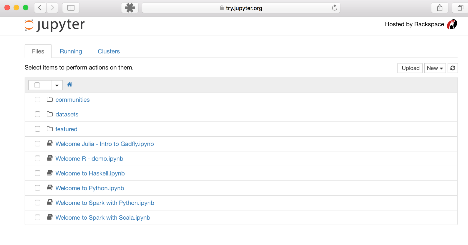
Jupyter Notebook App UI on Try Jupyter
Click on the New button on the top right, and choose "Python 3" from
the pull-down options to get a notebook that is connected to the IPython
kernel. You should get an empty notebook with a single empty code cell
labeled In[ ], with a flashing cursor inside. This is a code cell. You
can start by trying any simple mathematical operation (like a
calculator), and type [shift] + [enter] to execute it.
You can try any of the arithmetic operators in Python:
+ - * / ** % //
The last three operators above are exponent (raise to the power of),
modulo (divide and return remainder) and floor division. Be careful
that the division operator behaves differently in legacy Python 2: it
rounds to an integer when the operands are integers. We use Python 3 and
don't worry about this, because it gives the expected result, e.g.,
1/2 gives 0.5 (not zero!).
Here’s a simple example calculation in a code cell:
2 * 12
24
Typing [shift] + [enter] will execute the cell and give you the output
in a new line, labeled Out[1] (the numbering increases each time you
execute a cell). If you're at the end of the notebook, you will also
get a new blank cell, where you can try more arithmetic operations, if
you want. Or, you can change the type of cell from Code to Markdown
with the button on the menu bar. See if you find that now, and then type
some text into a markdwon cell. Try some markdown
syntax!
In a code cell, you can enter any valid Python code, and type
[shift] + [enter] to execute it. For example, the simplest code
example just prints the message Hello World!, like this:
print("Hello World!")
Hello World!
You can also define a variable (say x) and assign it a value (say, 2),
then use that variable in some code:
x = 2
print(x * "Hello World!")
Hello World!Hello World!
x * 12
24
More Jupyter cloud services
If you followed the instructions above, you launched the Jupyter
Notebook App on a cloud service called tmpnb. As the prefix tmp
indicates, it gives you a temporary demo: as soon as you close the
browser tab (or after a few minutes of inactivity), the kernel dies and
the content you wrote is not saved anywhere. This is a free service,
sponsored by the company Rackspace, just for trying something out.
You can work on notebooks and save your work using other cloud services. A long-running cloud offering is SageMathCloud. And most recently (in June 2016), Microsoft announced notebooks hosted on Azure cloud. In both cases, you need to create a free account to be able to save your work.
The world of Jupyter, so far
You learned about:
- the notebook,
- code cells and markdown cells,
- nbviewer,
- the Jupyter Notebook App,
[shift] + [enter]to execute,tmpnb, and- cloud notebook services.
Optional next step: local installation
Cloud notebook services (especially free ones!) have their limitations. As you start using notebooks more, you'll want to install Jupyter on your personal computer. For that, we recommend the free Anaconda distribution, which includes all the Python packages you may need (more than 700 packages are included!).
If you prefer a light installation (e.g., if your internet is slow), we
can recommend Miniconda. This
will include only conda (the package manager) and its dependencies,
and Python. You will have to install Jupyter separately, and also other
basic Python libraries for numerical mathematics and data analysis,
using the conda install command.
We also recommend that you start with Python 3 right away—Python 2.7 is the legacy Python, and you should only need to use it if you have a lot of code written in the past that you need to work with.
Read Conda Tutorial
The Python world of science and data
The Jupyter notebook is a nice way to write and share some content online, but you'll get superpowers from Python libraries for science and data!
We already used code cells to do simple calculations via the arithmetic operators in Python:
+ - * / ** % //
In addition to arithmetics, you can do comparisons with operators that
return Boolean values (True or False). These are:
== != < > <= >=
On top of those, you have assignment operators, bitwise operators, logical operators, membership operators, and identity operators. You can find online several "cheat sheets" for Python operators. For example: "Operators and expressions" in the online book "Python for You and Me."
Go ahead and experiment with various Python operators until you're
satisfied. You can open a new, empty notebook and experiment in code
cells, taking notes of the things that you find interesting in markdown
cells. Or, if you have this notebook open in the Jupyter Notebook App,
you can add a new cell by clicking the plus button,
and work right here. Remember to type [shift] + [enter] to execute any
cell.
Next, let’s learn about the Python world of science and data.
Two libraries that made Python useful for science: NumPy and Matplotlib
Python is a general-purpose language: you can use it to create websites, to write programs that crawl the web, to support you in scientific research or data analysis, etc. Because it can be used in so many fields, the core language is supported by many libraries (not everyone needs to have every functionality). In science, two libraries made Python really useful: NumPy and Matplotlib.
NumPy gives you access to numerical mathematics on arrays (like vectors and matrices). Matplotlib gives you a catalog of plotting functions for visualizing data.
import numpy
The command import followed by the name of a library will extend your
Python session with all of the functions in that library. After
executing the code cell above, we have all of NumPy available to us.
If you have this notebook open in the Jupyter Notebook App, make sure to
execute the cell above by clicking on it and typing [shift] + [enter].
Now, to use one of NumPy’s functions, we prepend numpy. (with the
dot) to the function name. For example:
numpy.linspace(0, 5, 10)
Output
array([ 0.        ,  0.55555556,  1.11111111,  1.66666667,  2.22222222,
        2.77777778,  3.33333333,  3.88888889,  4.44444444,  5.        ])
The NumPy function
linspace()
creates an array with equally spaced numbers between a start and end.
It’s a very useful function! In the code cell above, we create an array
of 10 numbers from 0 to 5. Go ahead and try it with different argument
values.
To be able to do something with this array later, we normally want to give it a name. Like,
xarray = numpy.linspace(0, 5, 10)
Now, we can use NumPy to do computations with the array. Like take its square:
xarray ** 2
Output
array([  0.        ,   0.30864198,   1.2345679 ,   2.77777778,
         4.9382716 ,   7.71604938,  11.11111111,  15.12345679,
        19.75308642,  25.        ])
In NumPy, the square of an array of numbers takes the square of each element. You will likely want to give your result a name, too. So let’s do this again, and also take the cube, and the square root of the array at the same time.
yarray = xarray ** 2
zarray = xarray ** 3
warray = numpy.sqrt(xarray)
You notice that NumPy knows how to take the power of an array, and
it has a built-in function for the square-root. Now, you may want to
draw a plot of these results with the original array on the x-axis. For
that we need the module pyplot from Matplotlib.
from matplotlib import pyplot
%matplotlib notebook
The command %matplotlib notebook is there to get our plots inside the
notebook (instead of a pop-up window, which is the default behavior of
pyplot). Let’s try a line plot now! We use the pyplot.plot()
function, specifying the line color ('k' for black) and line style
('-', '--' and ':' for continuous, dashed and dotted line), and
giving each line a label. Note that the values for color, linestyle
and label are given in quotes.
pyplot.plot(xarray,yarray,color='k',linestyle='-', label='square')
pyplot.plot(xarray,zarray,color='k',linestyle='--', label='cube')
pyplot.plot(xarray,warray,color='k',linestyle=':', label='square root')
pyplot.legend(loc='best')
pyplot.show()
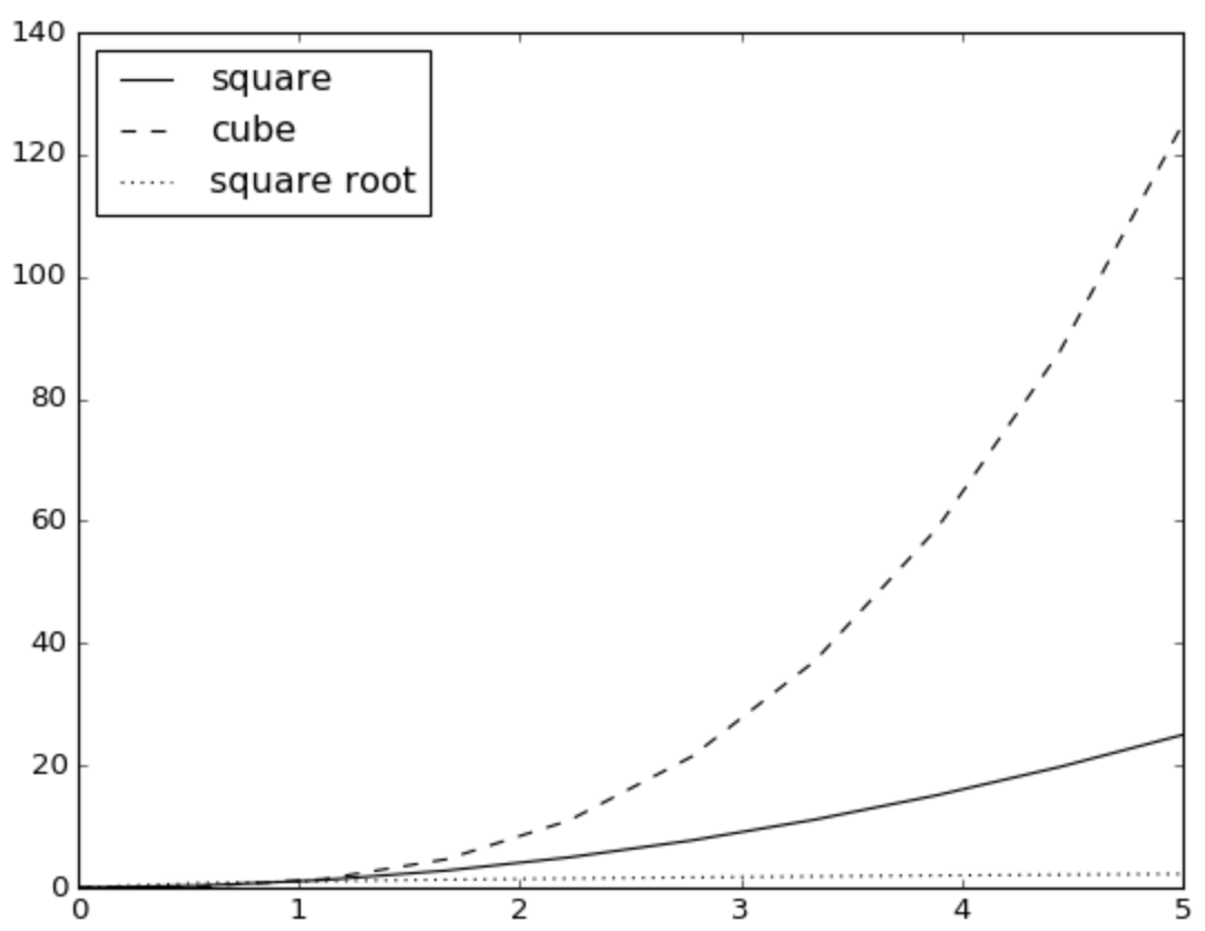
That’s very nice! By now, you are probably imagining all the great stuff you can do with Jupyter notebooks, Python and its scientific libraries NumPy and Matplotlib. Explore all the beautiful plots you can make by browsing the Matplotlib gallery.
Today, the world of Pyhon for science and data includes several other amazing libraries. For data analysis and modeling, you have pandas. For symbolic mathematics, SymPy gives you a Python-powered computer algebra system. You can draw beautiful 3D visualizations thanks to the Mayavi project. And there are many more!
The world of Python, so far
You learned about:
- Python operators
- the
importstatement - the NumPy library for array mathematics
- the Matplotlib library for plotting
- calling library functions by prepending the library name with a dot,
e.g.,
numpy.linspace() - making a line plot
- there’s a world of Python libraries for science and data
Optional next step: explore published notebooks
There are many ways you can go from here. To whet your appetite, you could browse for a bit on the Gallery of Interesting IPython Notebooks. Find a topic that interests you and see if there is a notebook that someone has shared; study the code examples and see if you can replicate some of it on your own fresh notebook.
If you would like to follow a step-by-step tutorial that teaches a foundation in computational fluid dynamics, let me introduce you to our very own "CFD Python. 12 steps to Navier-Stokes" — you can follow this 12-step program to build a solution to the Navier-Stokes equations for 2D cavity flow and 2D channel flow, using the finite-difference method.
Jupyter like a pro
In this third section, we want to leave you with pro tips for using Jupyter in your future work.
Importing libraries
First, a word on importing libraries. Previously, we used the following command to load all the functions in the NumPy library:
import numpy
Once you execute that command in a code cell, you call any NumPy
function by prepending the library name, e.g., numpy.linspace(),
numpy.ones(),
numpy.zeros(),
numpy.empty(),
numpy.copy(),
and so on (explore the documentation for these very useful functions!).
But, you will find a lot of sample code online that uses a different syntax for importing. They will do:
import numpy as np
All this does is create an alias for numpy with the shorter string
np, so you then would call a NumPy function like this:
np.linspace(). This is just an alternative way of doing it, for lazy
people that find it too long to type numpy and want to save 3
characters each time. For the not-lazy, typing numpy is more readable
and beautiful. We like it better like this:
import numpy
Make your plots beautiful
When you make a plot using Matplotlib, you have many options to make your plots beautiful and publication-ready. Here are some of our favorite tricks.
First, let’s load the pyplot module—and remember,
%matplotlib notebook gets our plots inside the notebook (instead of a
pop-up).
Our first trick is rcparams: we use it to customize the appearance of
the plots. Here, we set the default font to a serif type of size 14 pt
and make the size of the font for the axes labels 18 pt. Honestly, the
default font is too small.
from matplotlib import pyplot
%matplotlib notebook
pyplot.rcParams['font.family'] = 'serif'
pyplot.rcParams['font.size'] = 14
pyplot.rcParams['axes.labelsize'] = 18
The following example is from a tutorial by Dr. Justin Bois, a lecturer in Biology and Biological Engineering at Caltech, for his class in Data Analysis in the Biological Sciences (2015). He has given us permission to use it.
## Get an array of 100 evenly spaced points from 0 to 2*pi
x = numpy.linspace(0.0, 2.0 * numpy.pi, 100)

## Make a pointwise function of x with exp(sin(x))
y = numpy.exp(numpy.sin(x))
Here, we added comments in the Python code with the # mark. Comments
are often useful not only for others who read the code, but as a "note
to self" for the future you!
Let’s see how the plot looks with the new font settings we gave Matplotlib, and make the plot more friendly by adding axis labels. This is always a good idea!
pyplot.figure()
pyplot.plot(x, y, color='k', linestyle='-')
pyplot.xlabel('$x$')
pyplot.ylabel('$\mathrm{e}^{\sin(x)}$')
pyplot.xlim(0.0, 2.0 * numpy.pi);
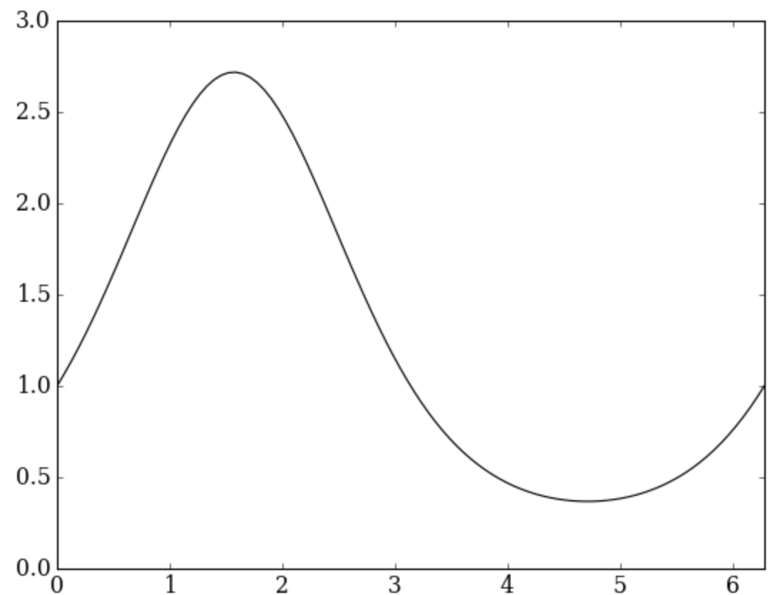
Did you see how Matplotlib understands LaTeX mathematics? That is
beautiful. The function pyplot.xlim() specifies the limits of the
x-axis (you can also manually specify the y-axis, if the defaults are
not good for you).
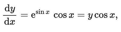
Continuing with the tutorial example by Justin Bois, let’s have some
mathematical fun and numerically compute the derivative of this
function, using finite differences. We need to apply the following
mathematical formula on all the discrete points of the x array:
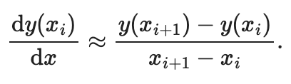
By the way, did you notice how we can typeset beautiful mathematics within a markdown cell? The Jupyter notebook is happy typesetting mathematics using LaTeX syntax.
Since this notebook is "Jupyter like a pro," we will define a custom Python function to compute the forward difference. It is good form to define custom functions to make your code modular and reusable.
def forward_diff(y, x):
    """Compute derivative by forward differencing."""

    # Use numpy.empty to make an empty array to put our derivatives in
    deriv = numpy.empty(y.size - 1)

    # Use a for-loop to go through each point and compute the derivative.
    for i in range(deriv.size):
        deriv[i] = (y[i+1] - y[i]) / (x[i+1] - x[i])

    # Return the derivative (a NumPy array)
    return deriv

## Call the function to perform finite differencing
deriv = forward_diff(y, x)
Notice how we define a function with the def statement, followed by
our custom name for the fuction, the function arguments in parenthesis,
and ending the statement with a colon. The contents of the function are
indicated by the indentation (four spaces, in this case), and the
return statement indicates what the function returns to the code that
called it (in this case, the contents of the variable deriv). Right
after the function definition (in between triple quotes) is the
docstring, a short text documenting what the function does. It is good
form to always write docstrings for your functions!
In our custom forward_diff() function, we used numpy.empty() to
create an empty array of length y.size-1, that is, one less than the
length of the array y. Then, we start a for-loop that iterates over
values of i using the
range()
function of Python. This is a very useful function that you should think
about for a little bit. What it does is create a list of integers. If
you give it just one argument, it’s a "stop" argument:
range(stop) creates a list of integers from 0 to stop-1, i.e., the
list has stop numbers in it because it always starts at zero. But you
can also give it a "start" and "step" argument.
Experiment with this, if you need to. It’s important that you
internalize the way range() works. Go ahead and create a new code
cell, and try things like:
for i in range(5):
   print(i)
changing the arguments of range(). (Note how we end the for
statement with a colon.) Now think for a bit: how many numbers does the
list have in the case of our custom function forward_diff()?
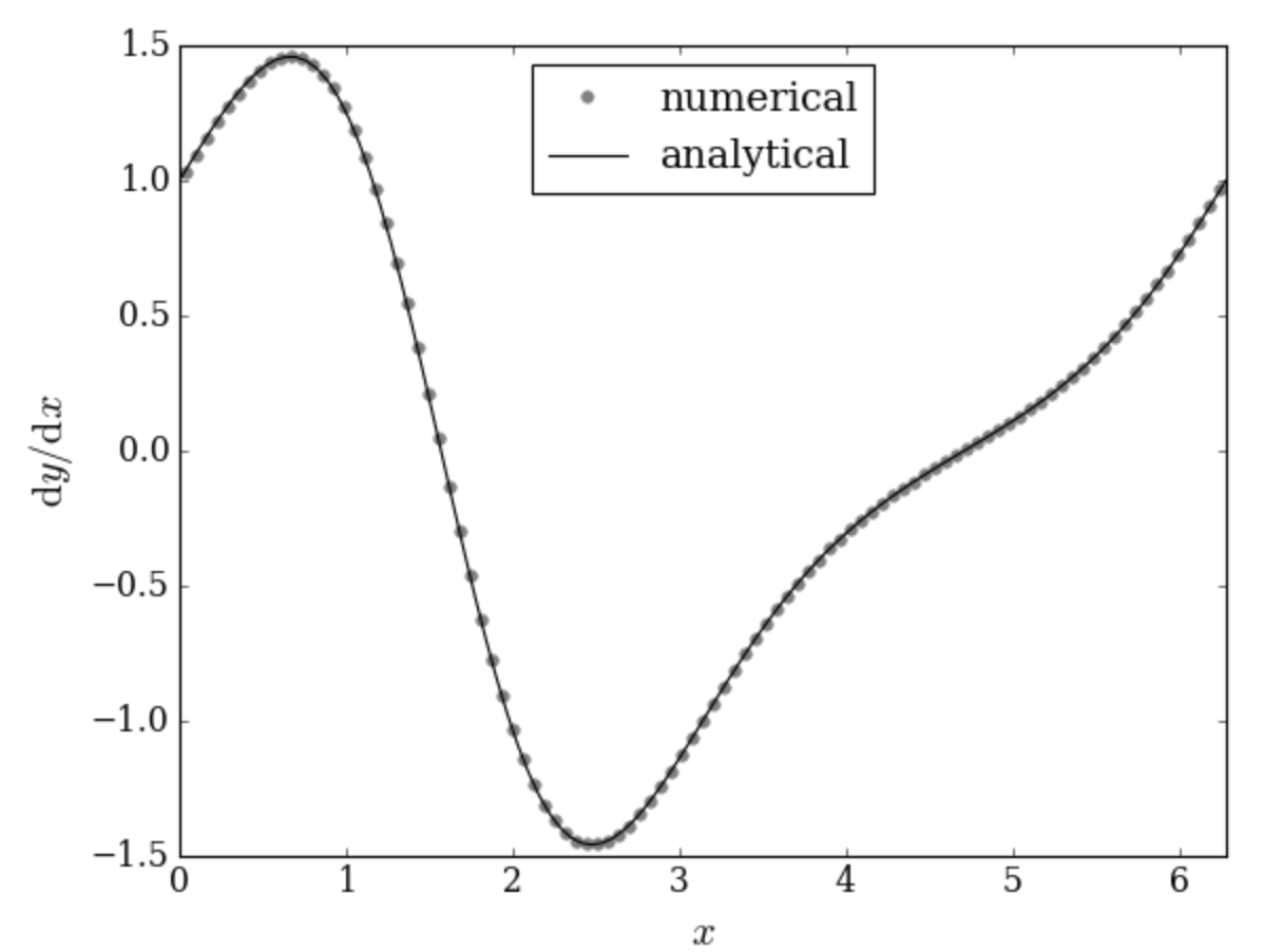
Now, we will make a plot of the numerical derivative of \(\exp(\sin(x))\). We can also compare with the analytical derivative:
deriv_exact = y * numpy.cos(x) # analytical derivative

pyplot.figure()
pyplot.plot((x[1:] + x[:-1]) / 2.0, deriv,
            label='numerical',
            marker='.', color='gray',
            linestyle='None', markersize=10)
pyplot.plot(x, deriv_exact,
            label='analytical',
            color='k', linestyle='-') # analytical derivative in black line

pyplot.xlabel('$x$')
pyplot.ylabel('$\mathrm{d}y/\mathrm{d}x$')
pyplot.xlim(0.0, 2.0 * numpy.pi)
pyplot.legend(loc='upper center', numpoints=1);
Stop for a bit and look at the first pyplot.plot() call above. The
square brackets normally are how you access a particular element of an
array via its index: x[0] is the first element of x, and x[i+1] is
the i-th element. What’s very cool is that you can also use
negative indices: they indicate counting backwards from the end of the
array, so x[-1] is the last element of x.
A neat trick of arrays is called
slicing:
picking elements using the colon notation. Its general form is
x[start:stop:step]. Note that, like the range() function, the stop
index is exclusive, i.e., x[stop] is not included in the result.
For example, this code will give the odd numbers from 1 to 7:
x = numpy.array( [0, 1, 2, 3, 4, 5, 6, 7, 8, 9] )
x[1:-1:2]
Try it! Remember, Python arrays are indexed from 0, so x[1] is the
second element. The end-point in the slice above is index -1, that’s
the last array element (not included in the result), and we're stepping
by 2, i.e., every other element. If the step is not given, it
defaults to 1. If start is not given, it defaults to the first array
element, and if stop is not given, it defaults to the last element.
Try several variations on the slice, until you're comfortable with it.
There’s a built-in for that
Here’s another pro tip: whenever you find yourself writing a custom
function for something that seems that a lot of people might use, find
out first if there’s a built-in for that. In this case, NumPy does
indeed have a built-in for taking the numerical derivative by
differencing! Check it out. We also use the function
numpy.allclose()
to check if the two results are close.
numpy_deriv = numpy.diff(y) / numpy.diff(x)
print('Are the two results close? {}'.format(numpy.allclose(numpy_deriv, deriv)))
Output
Are the two results close? True
Not only is the code much more compact and easy to read with the built-in NumPy function for the numerical derivative ... it is also much faster:
%timeit numpy_deriv = numpy.diff(y) / numpy.diff(x)
%timeit deriv = forward_diff(y, x)
Output
100000 loops, best of 3: 13.4 µs per loop
10000 loops, best of 3: 75.2 µs per loop
NumPy functions will always be faster than equivalent code you write yourself because at the heart they use pre-compiled code and highly optimized numerical libraries, like BLAS and LAPACK.
Do math like a pro
Do you want to compute the integral of \(y(x) = \mathrm{e}^{\sin x}\)? Of course you do. We find the analytical integral using the integral formulas for modified Bessel functions:
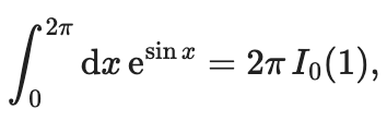
where \(I_0\) is the modified Bessel function of the first kind. But if
you don't have your special-functions handbook handy, we can find the
integral with Python. We just need the right modules from the
SciPy library.
SciPy has a module of special functions, including Bessel functions,
called scipy.special. Let’s get that loaded, then use it to compute
the exact integral:
import scipy.special
exact_integral = 2.0 * numpy.pi * scipy.special.iv(0, 1.0)

print('Exact integral: {}'.format(exact_integral))
Output
Exact integral: 7.95492652101
Or instead, we may want to compute the integral numerically, via the trapezoid rule. The integral is over one period of a periodic function, so only the constant term of its Fourier series will contribute (the periodic terms integrate to zero). The constant Fourier term is the mean of the function over the interval, and the integral is the area of a rectangle: \(2\pi \langle y(x)\rangle_x\). Sampling \(y\) at \(n\) evenly spaced points over the interval of length \(2\pi\), we have:
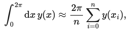
NumPy gives as a mean method to quickly get the sum:
approx_integral = 2.0 * numpy.pi * y[:-1].mean()

print('Approximate integral: {}'.format(approx_integral))
print('Error: {}'.format(exact_integral - approx_integral))
Output
Approximate integral: 7.95492652101
Error: 0.0
approx_integral = 2.0 * numpy.pi * numpy.mean(y[:-1])

print('Approximate integral: {}'.format(approx_integral))
print('Error: {}'.format(exact_integral - approx_integral))
Output
Approximate integral: 7.95492652101
Error: 0.0
The syntax y.mean() applies the mean() NumPy method to the array
y. Here, we apply the method to a slice of y that does not include
the last element (see discussion of slicing above). We could have also
done numpy.mean(y[:-1]) (the function equivalent of the method
mean() applied to an array); they give equivalent results and which
one you choose is a matter of style.
Beautiful interactive plots with Bokeh
Matplotlib will be your workhorse for creating plots in notebooks. But it’s not the only game in town! A recent new player is Bokeh, a visualization library to make amazing interactive plots and share them online. It can also handle very large data sets with excellent performance.
If you installed Anaconda in your system, you will probably already
have Bokeh. You can check if it’s there by running the conda list
command. If you installed Miniconda, you will need to install it
with conda install bokeh.
After installing Bokeh, we have many modules available:
bokeh.plotting
gives you the ability to create interactive figures with zoom, pan,
resize, save, and other tools.
from bokeh import plotting as bplotting
Bokeh integrates with Jupyter notebooks by calling the output function, as follows:
bplotting.output_notebook()
Output
BokehJS successfully loaded.
## create a new Bokeh plot with axis labels, name it "bop"
bop = bplotting.figure(x_axis_label='x', y_axis_label='dy/dx')

## add a title, change the font
bop.title = "Derivative of exp(sin(x))"
bop.title_text_font = "palatino"

## add a line with legend and line thickness to "bop"
bop.line(x, deriv_exact, legend="analytical", line_width=2)

## add circle markers with legend, specify color
bop.circle((x[1:] + x[:-1]) / 2.0, deriv, legend="numerical", fill_color="gray", size=8, line_color=None)

bop.grid.grid_line_alpha=0.3

bplotting.show(bop);
Note—As of June 2016 (v.0.11.1), Bokeh does not support LaTeX on axis labels. This is an issue they are working on, so stay tuned!
Look at the neat tools on the Bokeh figure: you can zoom in to any portion to explore the data, you can drag the plot area around, resize and finally save the figure to a file. You also have many beautiful styling options!
(C) CodeAhoy. Licensed under CC BY-SA 4.0.
Original content The world of Jupyter”—a tutorial. Used under Creative Commons Attribution License CC-BY 4.0.