Related Books


Books / The basics of R / Chapter 7
Web scrapping in R
Why scrape; Why not just copy and paste?
Imagine you want to collect information on the area and percentage water area of African countries. It’s easy enough to head to Wikipedia, click through each page, then copy the relevant information and paste it into a spreadsheet. Now imagine you want to repeat this for every country in the world! This can quickly become VERY tedious as you click between lots of pages, repeating the same actions over and over. It also increases the chance of making mistakes when copying and pasting. By automating this process using R to perform “Web Scraping,” you can reduce the chance of making mistakes and speed up your data collection. Additionally, once you have written the script, it can be adapted for a lot of different projects, saving time in the long run.
Web scraping refers to the action of extracting data from a web page using a computer program, in this case our computer program will be R. Other popular command line interfaces that can perform similar actions are wget and curl.
In this chapter
- this unordered seed list will be replaced by toc as unordered list
Getting started
Open up a new R Script where you will be adding the code for this tutorial. All the resources for this tutorial, including some helpful cheatsheets, can be downloaded from this Github repository. Clone and download the repo as a zipfile, then unzip and set the folder as your working directory by running the code below (subbing in the real path), or clicking Session/ Set Working Directory/ Choose Directory in the RStudio menu.
Alternatively, you can fork the repository to your own Github account and then add it as a new RStudio project by copying the HTTPS / SSH link. For more details on how to register on Github, download git, sync RStudio and Github and do version control.
setwd("<PATH TO FOLDER>")
1. Download the relevant packages
install.packages("rvest") # To import a html file
install.packages("dplyr") # To use pipes

library(rvest)
library(dplyr)
2. Download a .html web page
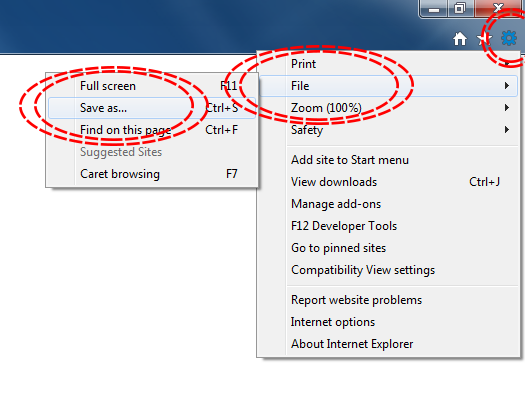
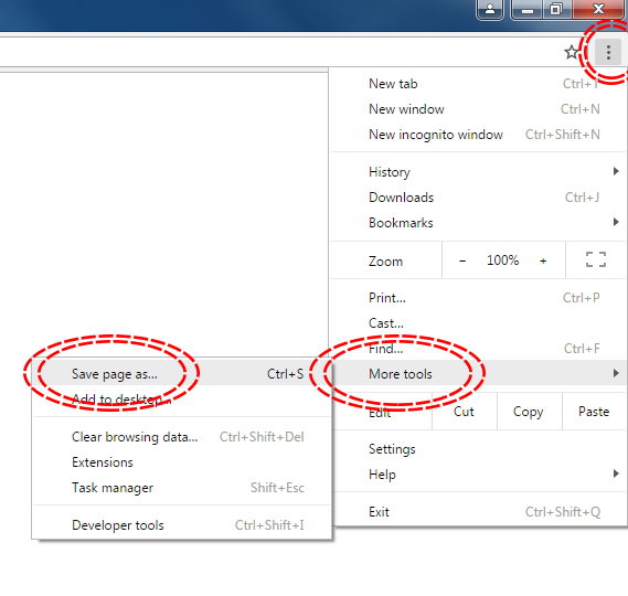
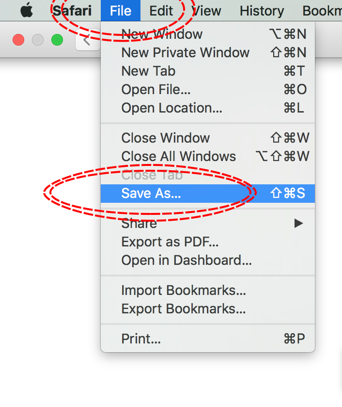
The simplest way to download a web page is to save it as a .html file to your working directory. This can be accomplished in most browsers by clicking File -> Save as... and saving the file type to Webpage, HTML Only or something similar. Here are some examples for different browser Operating System combinations:
Microsoft Windows - Internet Explorer
Microsoft Windows - Google Chrome
MacOS - Safari
Download the IUCN Red List information for Aptenogytes forsteri (Emperor Penguin) from [http://www.iucnredlist.org/details/22697752/0] using the above method, saving the file to your working directory.
3. Importing .html into R
The file can be imported into R as a vector using the following code:
Penguin_html <- readLines("Aptenodytes forsteri (Emperor Penguin).html")
Each string in the vector is one line of the original .html file.
4. Locating useful information using grep() and isolating it using gsub
In this example we are going to build a data frame of different species of penguin and gather data on their IUCN status and when the assessment was made so we will have a data frame that looks something like this:
| Scientific Name | Common Name | Red List Status | Assessment Date |
|---|---|---|---|
| Aptenodytes forsteri | Emperor Penguin | Near Threatened | 2016-10-01 |
| Aptenodytes patagonicus | King Penguin | Least Concern | 2016-10-01 |
| … | … | … | … |
| Spheniscus mendiculus | Galapagos Penguin | Endangered | 2016-10-01 |
Open the IUCN web page for the Emperor Penguin in a web browser. You should see that the species name is next to some other text, Scientific Name:. We can use this “anchor” to find the rough location of the species name:
grep("Scientific Name:", Penguin_html)
The code above tells us that Scientific Name: appears once in the vector, on string 132. We can search around string 132 to find the species name:
Penguin_html[131:135]
This displays the contents of our subsetted vector:
[1] "<tr>"
[2] "  <td class=\"label\"><strong>Scientific Name:</strong></td>"
[3] "  <td class=\"sciName\"><span class=\"notranslate\"><span class=\"sciname\">Aptenodytes forsteri</span></span></td>"
[4] "</tr>"
[5] ""
Aptenoydes forsteri is on line 133, wrapped in a whole load of html tags. Now we can check and isolate the exact piece of text we want, removing all the unwanted information:
# Double check the line containing the scienific name.
grep("Scientific Name:", Penguin_html)
Penguin_html[131:135]
Penguin_html[133]

# Isolate line in new vector
species_line <- Penguin_htm[133]

## Use pipes to grab the text and get rid of unwanted information like html tags
species_name <- species_line %>%
  gsub("<td class=\"sciName\"><span class=\"notranslate\"><span class=\"sciname\">", "", .) %>%  # Remove leading html tag
  gsub("</span></span></td>", "", .) %>%  # Remove trailing html tag
  gsub("^\\s+|\\s+$", "", .)  # Remove whitespace and replace with nothing
species_name
For more information on using pipes, follow our data manipulation tutorial.
gsub() works in the following way:
gsub("Pattern to replace", "The replacement pattern", .)
This is self explanatory when we remove the html tags, but the pattern to remove whitespace looks like a lot of random characters. In this gsub() command, we have used “regular expressions” also known as “regex”. These are sets of character combinations that R (and many other programming languages) can understand and are used to search through character strings. Let’s break down "^\\s+|\\s+$" to understand what it means:
^ = From start of string
\\s = White space
+ = Select 1 or more instances of the character before
| = “or”
$ = To the end of the line
So "^\\s+|\\s+$" can be interpreted as “Select one or more white spaces that exist at the start of the string and select one or more white spaces that exist at the end of the string”. Look in the repository for this tutorial for a regex cheat sheet to help you master grep.
We can do the same for common name:
grep("Common Name", Penguin_html)
Penguin_html[130:160]
Penguin_html[150:160]
Penguin_html[151]

common_name <- Penguin_html[151] %>%
  gsub("<td>", "", .) %>%
  gsub("</td>", "", .) %>%
  gsub("^\\s+|\\s+$", "", .)
common_name
IUCN category:
grep("Red List Category", Penguin_html)
Penguin_html[179:185]
Penguin_html[182]

red_cat <- gsub("^\\s+|\\s+$", "", Penguin_html[182])
red_cat
Date of Assessment:
grep("Date Assessed:", Penguin_html)
Penguin_html[192:197]
Penguin_html[196]

date_assess <- Penguin_html[196] %>%
	gsub("<td>", "",.) %>%
	gsub("</td>", "",.) %>%
	gsub("\\s", "",.)
date_assess
We can create the start of our data frame by concatenating the vectors:
iucn <- data.frame(species_name, common_name, red_cat, date_assess)
5. Importing multiple web pages
The above example only used one file, but the real power of web scraping comes from being able to repeat these actions over a number of web pages to build up a larger dataset.
We can import many web pages from a list of URLs generated by searching the IUCN red list for the word Penguin. Go to [http://www.iucnredlist.org], search for “penguin” and download the resulting web page as a .html file in your working directory.
Import Search Results.html:
search_html <- readLines("Search Results.html")
Now we can search for lines containing links to species pages:
line_list <- grep("<a href=\"/details", search_html)  # Create a vector of line numbers in `search_html` that contain species links
link_list <- search_html[line_list]  # Isolate those lines and place in a new vector
Clean up the lines so only the full URL is left:
species_list <- link_list %>%
  gsub('<a href=\"', "http://www.iucnredlist.org", .) %>%  # Replace the leading html tag with a URL prefix
  gsub('\".*', "", .) %>%  # Remove everything after the `"`
  gsub('\\s', "",.)  # Remove any white space
Clean up the lines so only the species name is left and transform it into a file name for each web page download:
file_list_grep <- link_list %>%
  gsub('.*sciname\">', "", .) %>% # Remove everything before `sciname\">`
  gsub('</span></a>.*', ".html", .) # Replace everything after `</span></a>` with `.html`
file_list_grep
Now we can use mapply() to download each web page in turn using species_list and name the files using file_list_grep:
mapply(function(x,y) download.file(x,y), species_list, file_list_grep)
mapply() loops through download.file for each instance of species_list and file_list_grep, giving us 18 files saved to the working directory
Import each of the downloaded .html files based on its name:
penguin_html_list <- lapply(file_list_grep, readLines)
Now we can perform similar actions to those in the first part of the tutorial to loop over each of the vectors in penguin_html_list and build our data frame:
Search for “Scientific Name:” and store the line number for each web page in a list:
sci_name_list_rough <- lapply(penguin_html_list, grep, pattern="Scientific Name:")
sci_name_list_rough
penguin_html_list[[2]][133]
Convert the list into a simple vector using unlist(). +1 gives us the line containing the actual species name rather than Scientific Name::
sci_name_unlist_rough <- unlist(sci_name_list_rough) + 1
Retrieve lines containing scientific names from each .html file in turn and store in a vector:
sci_name_line <- mapply('[', penguin_html_list, sci_name_unlist_rough)
Remove the html tags and whitespace around each entry:
## Clean html
sci_name <- sci_name_line %>%
  gsub("<td class=\"sciName\"><span class=\"notranslate\"><span class=\"sciname\">", "", .) %>%
  gsub("</span></span></td>", "", .) %>%
  gsub("^\\s+|\\s+$", "", .)
As before, we can perform similar actions for Common Name:
# Find common name
## Isolate line
common_name_list_rough <- lapply(penguin_html_list, grep, pattern = "Common Name")
common_name_list_rough #146
penguin_html_list[[1]][151]
common_name_unlist_rough <- unlist(common_name_list_rough) + 5
common_name_line <- mapply('[', penguin_html_list, common_name_unlist_rough)
common_name <- common_name_line %>%
  gsub("<td>", "", .) %>%
  gsub("</td>", "", .) %>%
  gsub("^\\s+|\\s+$", "", .)
Red list category:
red_cat_list_rough <- lapply(penguin_html_list, grep, pattern = "Red List Category")
red_cat_list_rough
penguin_html_list[[16]][186]
red_cat_unlist_rough <- unlist(red_cat_list_rough) + 2
red_cat_unlist_rough
penguin_html_list[[2]][187]
red_cat_line <- mapply(`[`, penguin_html_list, red_cat_unlist_rough)
red_cat <- gsub("^\\s+|\\s+$", "", red_cat_line)
Date assessed:
date_list_rough <- lapply(penguin_html_list, grep, pattern = "Date Assessed:")
date_list_rough  # Different locations
penguin_html_list[[18]][200]
date_unlist_rough <- unlist(date_list_rough) + 1
date_line <- mapply('[', penguin_html_list, date_unlist_rough)
date <- date_line %>%
  gsub("<td>", "",.) %>%
  gsub("</td>", "",.) %>%
  gsub("\\s", "",.)
Then we can combine the vectors into a data frame:
penguin_df <- data.frame(sci_name, common_name, red_cat, date)
penguin_df
Does your data frame look something like this?
| sci_name | common_name | red_cat | date |
|---|---|---|---|
| Aptenodytes forsteri | Emperor Penguin | Near Threatened | 2016-10-01 |
| Aptenodytes patagonicus | King Penguin | Least Concern | 2016-10-01 |
| Eudyptes chrysocome | Southern Rockhopper Penguin, Rockhopper Penguin | Vulnerable | 2016-10-01 |
| Eudyptes chrysolophus | Macaroni Penguin | Vulnerable | 2016-10-01 |
| Eudyptes moseleyi | Northern Rockhopper Penguin | Endangered | 2016-10-01 |
| Eudyptes pachyrhynchus | Fiordland Penguin, Fiordland Crested Penguin | Vulnerable | 2016-10-01 |
| Eudyptes robustus | Snares Penguin, Snares Crested Penguin, Snares Islands Penguin | Vulnerable | 2016-10-01 |
| Eudyptes schlegeli | Royal Penguin | Near Threatened | 2016-10-01 |
| Eudyptes sclateri | Erect-crested Penguin, Big-crested Penguin | Endangered | 2016-10-01 |
| Eudyptula minor | Little Penguin, Blue Penguin, Fairy Penguin | Least Concern | 2016-10-01 |
| Megadyptes antipodes | Yellow-eyed Penguin | Endangered | 2016-10-01 |
| Pygoscelis adeliae | Adélie Penguin | Least Concern | 2016-10-01 |
| Pygoscelis antarcticus | Chinstrap Penguin | Least Concern | 2016-10-01 |
| Pygoscelis papua | Gentoo Penguin | Least Concern | 2016-10-01 |
| Spheniscus demersus | African Penguin, Jackass Penguin, Black-footed Penguin | Endangered | 2016-10-01 |
| Spheniscus humboldti | Humboldt Penguin, Peruvian Penguin | Vulnerable | 2016-10-01 |
| Spheniscus magellanicus | Magellanic Penguin | Near Threatened | 2016-10-01 |
| Spheniscus mendiculus | Galapagos Penguin, Galápagos Penguin | Endangered | 2016-10-01 |
Now that you have your data frame you can start analysing it. Try to make a bar chart showing how many penguin species are in each red list category.
A full .R script for this tutorial along with some helpful cheatsheets and data can be found in the repository for this tutorial.