In my previous blog post, I claimed that “AI is not magic.” In this post, my goal is to discuss how neural networks learn, and show that AI isn’t a crystal ball or magic, just science and some very slick mathematics. I’ll keep this very high level.
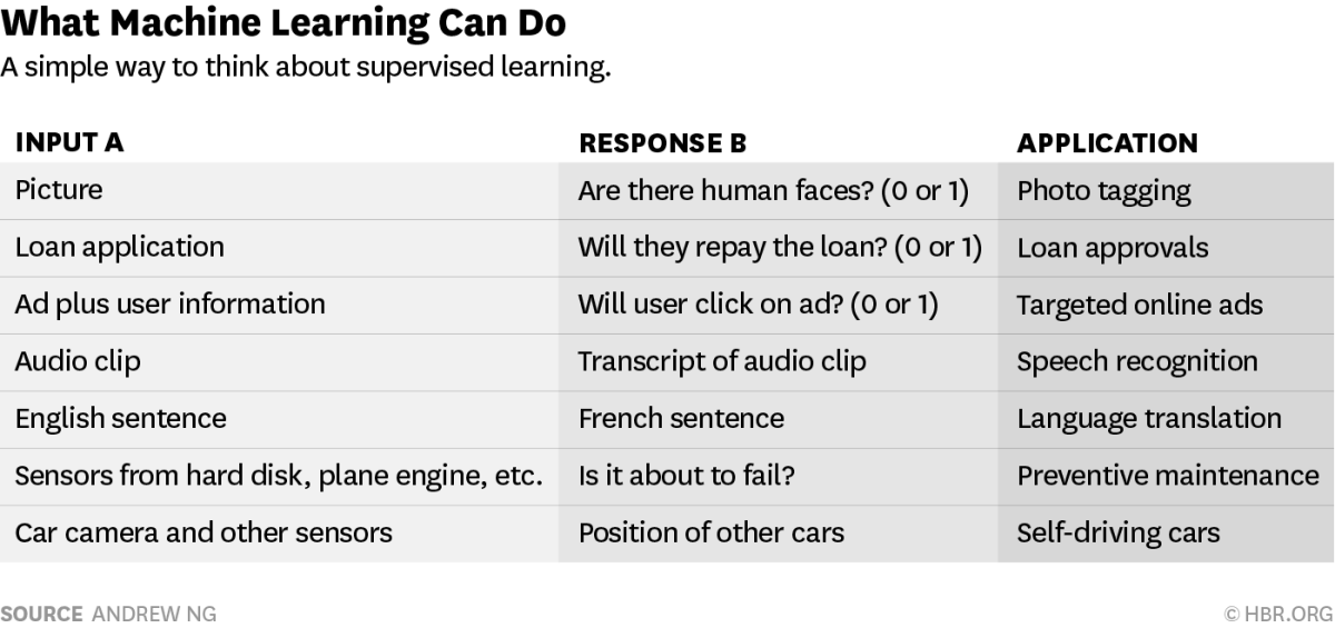
Let’s start with a hypothetical scenario. Suppose we are building an app to identify hot dogs. Take a picture and the app will tell you if it’s a hotdog or not. Total App Store domination.
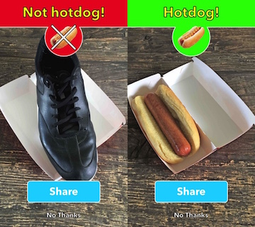
To recognize images, we choose to implement a popular machine learning algorithm called the neural network. (In this hypothetical scenario) This decision was made after reading an online article which talked about how neural networks can learn to recognize objects by training on lots of labelled examples. Once trained, it can start identifying images it has never seen before. We go ahead and obtain a training set of 6000 images gathered from online sources. 1000 images of different types of hotdogs: New York vs Chicago, ketchup, no ketchup, hotdogs on a grill, etc. The other 5000 images are of various non-hotdog objects: shoes, hamburgers, burrito, human legs. Now all that remains is to build our neural network.
To understand neural networks, we must first understand its elementary building block: the artificial neuron.
An artificial neuron takes one ore more inputs and produces a single output.
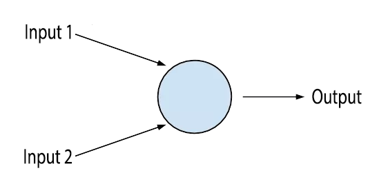
Looks familiar? It looks a lot like logic gates, which are elementary building blocks of digital circuits. The similarity ends there. Unlike logic gates, neurons can have several inputs and can change output for the same input values. This is possible because neurons have weights associated with each input, which is multiplied with the input value. These weights allow neurons to rate how important each input is. E.g. if the second input to a neuron isn’t very important, neuron can assign it a weight close to 0 essentially cancelling it out. Neurons also have biases which controls how easy it is to get neuron to output or fire. If the bias is huge, the neuron will fire very easily. I may have simplified, but what I have just described is the most basic type of neuron called the perceptron. In real world, we use more complex types of neurons.
An individual neuron is nifty, but it is not enough for sophisticated decision making. We want to group a bunch of these neurons together to form a neural network where different neurons get tuned on different aspects of the image. For example, a subset of neurons may only fire when they detect sliced bun, while others may fire when they detect sausage. All these sub decisions are weighed in the output layer before the final judgement is passed. For example, if the sausage neurons aren’t firing but the sliced bun one’s are, the output layer will classify the image as not hotdog because it could be something else with a sliced bun, e.g. Philly cheese steak sandwich. Output layer will assign more weight to the input coming from sausage neurons because there’s a very high chance that the image is of hotdog when the sausage neurons are firing.
When we connect bunch of neurons together, we get a neural network.
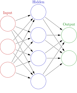
This particular type of neural network is called feedforward because information just flows in one direction and there are no cycles. Let’s also quickly talk about how we’ll input images to our neural network. Suppose that all images are the same resolution, say 128 by 128 pixels. We represent each image as a 2d array where each element of the array contains color information for the corresponding pixel. This 2d array of pixel color values is fed to the input layer of our neural network which contains 128*128=16384 neurons.
Back to weights and biases. The ability to change output for the same input values is arguably the most important feature of an artificial neuron (and by extension, the neural network) and it is the key to its learning. The goal of learning is to find the best combination of weights and biases for the neural network. Let’s express this objective formally so we can measure it and give it a name: cost function:
Cost Function (weights,biases) = (# of images incorrectly identified) ÷ (Total # of images)
Great. Now we can measure the performance with a clear objective: find weights and biases which minimize the cost function. How to find best weights and biases? One way is to just randomly pick them, run neural network over entire training data (6,000 images) and calculate the cost function which is the ratio of images incorrectly identified and the total number of images. Keep repeating until we’ve found a low enough value of the cost function that we like. Let’s say we want to stop when the neural network has a success rate of 99%. When we reach this goal, the combination of weights and biases reflect some similarity between hotdogs and our neural network can identify never seen before hotdog images. Let’s try it out. To keep it simple, suppose we are only doing this for 2 weights and biases.
Iteration 1: Weight1 = 1, Weight2 = 3, Bias1 = 1, Bias2 = 4. Let’s say it correctly classifies 300 out of 500 images of hot dog correctly. We’ll say the error rate is 200/500 = 40%
Iteration 2: Weight1 = 14, Weight2 = 6, Bias1 = 3, Bias2 = 0.2. This time is classifies 250 out of 500 images of hot dog correctly. The error rate is 200/500 = 50%, worst than last time.
Iteration 3: Choose weights and biases randomly again, roll the dice and error rate is 35%. Hmmm…
…
I hope you can see why this approach won’t work. There is no science, even heuristics to it. If the luck isn’t on our side, we could keep iterating until the end of time. And this is with just 2 weights and biases. In reality, it’s not uncommon for neural networks to have hundreds or even thousands of weights and biases. The shot in the dark approach just isn’t practical, it’s impossible.
But thanks to mathematics and calculus, we have a way of finding optimum weights and biases quicker, or in other words, minimizing the cost function in a scientific manner. This is done using an algorithm called the ‘Gradient Descent.’ The first time it runs, the algorithm picks up random weights and biases, but in subsequent iterations, it doesn’t chooses randomly but in a calculated manner to minimize the cost function even further. It keeps iterating until it finds the minimum value of the cost function. At this point, our neural network is said to have been ‘trained’ and it could start classifying pictures that it hasn’t seen before.
Of course, there is much, much more happening under the hood. If you are interested, Andrew Ng has an excellent lecture on gradient descent and I encourage you to watch the video so understand it in more detail.
Let’s revisit our cost function:
Cost Function (weights,biases) = (# of images incorrectly identified) ÷ (Total # of images)
This cost function is too simple and isn’t practical for gradient descent. Gradient descent cannot make incremental updates to weights and biases to minimize it. We need a smooth cost function. In practice, people usually use a quadratic cost function also known as the mean squared error (MSE).

Here Ŷ is the prediction of the learning algorithm, Y is the actual value and n is the size of the training data. It’s a measure of how close predictions are to actual values. Data scientists often multiply the cost function by 1/2 because that way the squared term is easier to cancel when taking derivative of the function. Speaking of derivative, gradient descent minimizes the cost function by taking its derivative (slope at that point) and moving in the direction where it is decreasing.
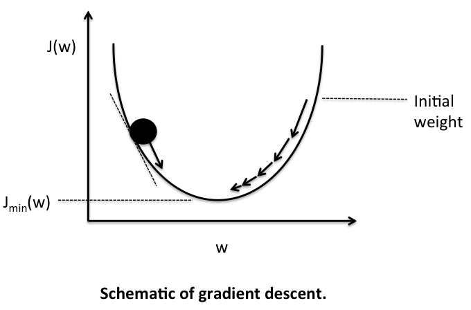
Unlike the first simplified cost function we created, MSE is a smooth cost function. In each iteration, gradient descent updates weights and biases to move downhill to the lowest point where the cost function is minimum. As a side note, there are many types of cost functions but MSE works well in many cases.
There is one more concept that you should know: the learning rate. The learning rate is the amount by which gradient descent updates weights and biases in each step. If the learning rate is too low, the algorithm may take a very long time to find the minimum. If the learning rate is too high, the algorithm may overshoot and miss the minimum (i.e. jump to the other side of the hill.) In practice, several parameters like learning rate and others that we’ll see in later posts needs to be adjusted to get the best results and performance.
Gradient descent, or rather its variations and several optimizations (as we’ll see in later posts), remains in wide use in machine learning algorithms like linear regression and neural networks. In linear regression, it gives us the line that best fits the data we are modeling; in neural networks, it gives us the best weights and biases.
Is AI magic? Magic of matrix multiplication and gradient descent, sure. But not smart enough to take over and destroy the world. Many CEO’s and executives overestimate the power of AI because of the unrealistic picture painted by the media. AI is extremely powerful and is proving itself with positive ROI in many domains, but it also has its limitations and it is not an off-the-shelf crystal ball. You should understand what the AI can and cannot do and then incorporate into your overall strategy. A good rule of thumb:
If a typical person can do a mental task with less than one second of thought, we can probably automate it using AI either now or in the near future. (-Andrew Ng)
See you next time.