Related Books


Books / Graph Algorithms / Chapter 7
Shortest Path Algorithms - Single Source Shortest Path
We assume that the graphs in question are directed graphs. There are a few different types of shortest path problems. The simplest one is the single-source shortest path problem. The most general statement of the problem is the shortest weighted path problem. This is one of the hardest versions of the problem. A weighted path is a path in a weighted graph. The weight of a path is the sum of the weights of the edges on the path. A weighted path from a vertex s to a vertex v is a shortest weighted path if there is no other path in the graph from s to v that has shorter weight. For convenience, when we say a shortest path we mean a shortest weighted path, not a path with the fewest edges. The distance between two vertices is the weight of a shortest path between the vertices.
The shortest path problem is the problem of finding a path between two vertices (or nodes) in a graph such that the sum of the weights of its constituent edges is minimized. For example, finding the shortest path between two intersections on a road.
Single Source Shortest Path Problem
Given a weighted graph G = (V, E), and a distinguished vertex s, find the shortest weighted path between s and every other vertex in the graph.
If we let the weight of every edge be 1, then this statement of the problem is reduced to finding the paths whose lengths are least. Edgar Dijkstra proposed an algorithm to solve the weighted graph version of this problem provided that edges do not have negative edge weights. In his algorithm, it does not matter whether the graph is directed or undirected. The output of the algorithm is a list of the shortest (weighted) distances to each vertex. If the output needs to include the set of paths to each vertex, then the algorithm can be modified to record this information.
The idea of the algorithm is to maintain a temporary set of vertices, T, with the property that the shortest path from s to every vertex in T has been correctly determined, and to enlarge this set iteratively. This set can be thought of as the known set, because for any vertex in this set, the shortest path from s to that vertex is known to be correct. Initially, only the source vertex s will be in T, since the distance from s to s is 0. In each iteration, a new vertex is added to T. When the size of the known set is equal to |V| , the algorithm stops.
The algorithm also maintains, for each vertex v not in T, a temporary least distance, d(v), from s. The value d(v) is the weight of the shortest path from s to v that, except for v, passes only through vertices in T. The algorithm may discover as it proceeds that d(v) is too large, and it will reduce it when that happens. We call d(v) an estimated distance.
After initializing the set T and recording the initial estimated distances d(v) to each node, the algorithm enters a loop. In each iteration of the loop, a vertex v ∈ V − T with minimal d(v) is added to T, and the distances d(u) to each u ∈ V − T are updated. Since the set T starts with just the vertex s in it, and in each iteration, a vertex that is not in T is added to it, the algorithm must iterate exactly |V − 1| times, and after |V − 1| iterations of the loop, all vertices have been added to T and the algorithm terminates.
In the description of the algorithm that follows, we assume first that the cost of each edge is denoted by a cost function c(v, w), which is defined on each edge (v, w) in the edge set E. This function needs to be extended to a function c’(v, w) that is defined on all pairs of vertices v, w ∈ V as follows, even if there is no edge (v, w) in E. This function is defined as follows:
\[c^{\prime}(v, w)= \begin{cases}0 & \text { if } v=w \\ c(v, w) & \text { if } v \neq w \wedge(v, w) \in E \\ \infty & \text { if } v \neq w \wedge(v, w) \notin E\end{cases}\]In other words, the cost of an edge (v, w) is infinite if the edge does not exist. In an actual implementation, a special value could denote when an edge does not exist. The cost of all other edges is simply the weight of the edge itself.
Algorithm
The following listing is a pseudocode description of the algorithm:
 // Initialize the function d(v) by setting d(v) to the cost of
 // the edge from s to v and setting d(s) to 0:

 for each v in V {
   d(v) = c'(s , v ) ; // set initial distances
 }

 // Implies that d(s) has been set to 0

 // Initialize the set T to contain only the vertex s
 T = {
   s
 };

 // Iterate until every vertex from V has been added to T
 while (T != V) {
   choose a vertex v in V - T with least d(v);
   set T = T + {
     v
   }; // add v to T
   // update the distances from s to each vertex not yet placed
   // into T. The only vertices whose distance might change are
   // the ones that are adjacent to v.
   for all vertices u in V - T that are adjacent to v {
     // if the current distance to u is larger than the
     // distance from s to v and then from v to u, then
     // replace d(u) by the new, smaller distance.
     if (d(u) > d(v) + c'(v , u))
       d(u) = d(v) + c'(v , u) ;
     }
   }
When we find the vertex v whose d(v) is minimal among all vertices not yet in T, we look at all vertices adjacent to it, and for each one u, if the weight of the path from s to u going through v is less than it was without going through v, we decrease the weight of its potential shortest path so that it is the weight of the path from s to u through v.
Example
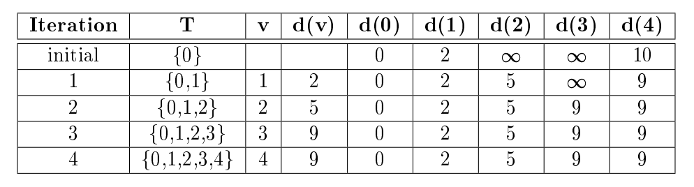
Given the graph in Figure 2, the table below shows how the set T and the values d(v) change in each iteration when s = 0. The columns show the state at the end of the iteration, not before.
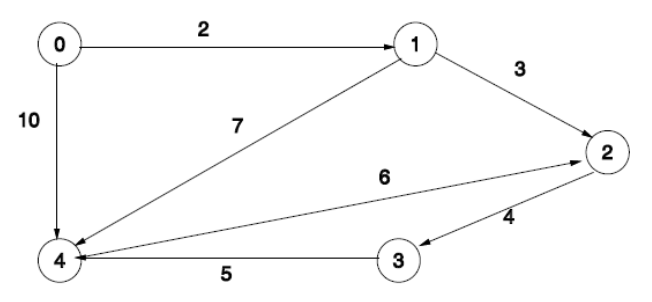
Figure 2: Example for Dijkstra’s Algorithm.
Implementation Issues
The graph should be represented by an adjacency list, because within the loop, we have to find the set of nodes adjacent to the chosen vertex v. An adjacency list representation makes it possible to visit the nodes that are adjacent to v in constant time. I.e., if there are m nodes adjacent to v, it will take m steps to visit them.
Most graphs are sparse - the number of edges is roughly |V| . For these graphs, it makes sense to use a priority queue to store the vertices in V − T, and to use a deleteMin operation to pick the vertex from V − T whose distance d(v) is smallest. We do not need to create an actual set T; we can maintain a boolean array with an entry for each vertex in V ; the entry would be false if v is not in T and true if it is in T. To decide whether a vertex u that is adjacent to v is in the set T, we just inspect its boolean value in this array.
The hard part is efficiently updating the function d(v) for all vertices not in T. Suppose that we use a binary heap for the priority queue. If we assume that the adjacency list entry for a vertex stores the index of the vertex in the binary heap, or -1 if it is not in the heap, then each time that we need to decrease the value of d(u) for a vertex u that is adjacent to v and in the heap, we look up its index in the heap from the adjacency list, e.g.
k = A[u].heapindex;
and then modify the value of d(u) in the heap with something like:
heap[k].distance = *d(v)* + c'(v,u);
where the right hand side is the distance from s to v plus the weight of the edge from v to u, obtained from the adjacency list. Now this is not enough, as the heap element has changed value and must be percolated up. So we follow the update with a percolateUp operation.