Related Books


Books / Graph Algorithms / Chapter 8
Shortest Path Algorithms - All-Pairs Shortest Path
The All-Pairs Shortest Path Problem
Sometimes we want to compute the shortest paths between all pairs of vertices. One example of this is in producing a chart that contains the minimum distances or costs of traveling between any pair of cities in a given geographic region:
Let G = (V, E) be the graph in which V is the set of all American cities with airports, and E is the set of all edges (v, w) such that there is a scheduled flight from city v to city w by some commercial airline. The weight c(v, w) assigned to the edge (v, w) might be:
- the air distance between v and w,
- the air time between them, or
- the price of a minimum price ticket.
The weights associated with edges might be travel time or the cost of an airline ticket. For this reason the pairs are ordered pairs, since these costs are not symmetric, and the collection of cities with inter-city distances will be represented by a weighted, directed graph.
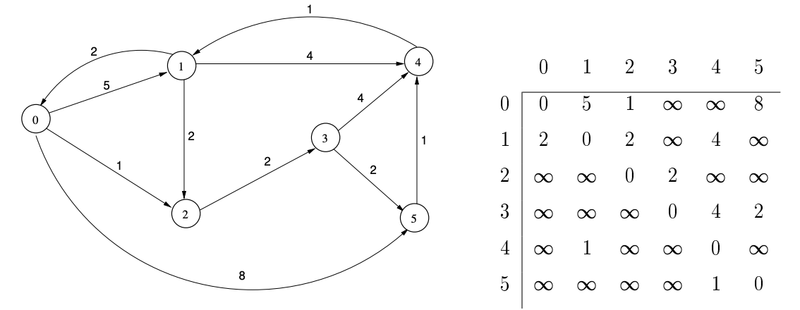
Figure 1: A weighted, directed graph and its adjacency matrix representation.
Figure 1 contains a weighted, directed graph. It shows that the distance from vertex 0 to vertex 1 is 5, for example, and that the direct distance from vertex 3 to vertex 4 is 4. But notice that the distance from vertex 3 to vertex 4 obtained by traveling through vertex 5 is 1 + 2 = 3, illustrating that the shortest distance between two vertices is not necessarily the one along the least number of edges. The all-pairs, shortest-path problem is, given a graph G, to find the lengths of the shortest paths between every pair of vertices in the graph.
The first step in designing an algorithm to solve this problem is deciding which representation to use for the graph. For this particular problem, the best representation is an adjacency matrix, which we denote A**. If the graph has an edge *(i, j), then \(A_{i, j}\) will be the weight of the edge. If there is no edge, conceptually we want to assign \(\infty\) to the entry \(A_{i, j}\). When we do arithmetic, we would use the rule that \(\infty+c=\infty\) for all constants \(c\). In Figure 1 the adjacency matrix has \(\infty\) in all entries that correspond to non-existent edges. In an actual application, we would have to use a very large number instead of \(\infty\).
The adjacency matrix representation uses an amount of storage proportional to \(O\left(V^{2}\right)\). Other graph representations use storage that is asymptotically smaller. When the graph is sparse, meaning that the number of edges is small in comparison to \(n^{2}\), this representation may not be suitable. But for this particular problem, the big advantage is that it is constant time access to each edge weight, and this advantage outweighs the high cost of storage. This is why we say it is the best representation in this case. A convenience of using the matrix is that we can use it to store the final, shortest distances between all pairs of vertices. In other words, when the algorithm terminates, the matrix entry \(A_{i j}\) will contain the shortest distance between vertex i and vertex j.
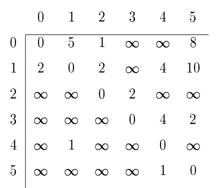
Table 1: The shortest paths matrix after one iteration.
There are several different algorithms to solve this problem; however, we will present Floyd’s algorithm. Floyd’s algorithm is also known as the Floyd-Warshall algorithm. It was discovered independently by Robert Floyd and Stephen Warshall in 1962 This algorithm has one restriction: it will not work correctly if there are negative cycles in the graph. A negative cycle is a cycle whose total edge weight is negative. We will assume there are no such cycles in our graph. After all, distances between cities cannot be negative. Floyd’s algorithm runs in \(\Theta\left(V^{3}\right)\) time regardless of the input, so its worst case and average case are the same. A pseudo-code description is in Listing 1 below.
// let A be a n by n adjacency matrix
for k = 0 to n -1 {
    for i = 0 to n -1 {
        for j = 0 to n -1 {
            if (A [i , j ] > A [i , k ] + A [k , j ]) {
                A [i , j ] = A [i , k ] + A [k , j ];
            }
        }
    }
}
Initially, the length of the shortest path between every pair of vertices i and j is just the weight of the edge from i to j stored in \(A[i, j]\). In each iteration of the outer loop, every pair of vertices (i, j) is checked to see whether there is a shorter path between them that goes through vertex \(k\) than is currently stored in the matrix. For example, when \(\mathrm{k}=0\), the algorithm checks whether the path from i to 0 and then 0 to j is shorter than the edge (i, j), and if so, \(A[i, j]\) is replaced by the length of that path. It repeats this for each successive value of \(\mathrm{k}\). With the graph in Figure 1 until \(\mathrm{k}=5\), the entry \(\mathrm{A}[3,4]\) has the value 4 , as this is the weight of the edge \((3,4)\). But when \(\mathrm{k}=5\), the algorithm will discover that \(\mathrm{A}[3,5]+\mathrm{A}[5,4]<\mathrm{A}[3,4]\), so it will replace \(\mathrm{A}[3,4]\) by that sum. In the end, the lengths of the shortest paths have replaced the edge weights in the matrix. Note that this algorithm does not tell us what the shortest paths are, only what their lengths are. The result of applying Floyd’s algorithm to the matrix in Figure 1 is shown in Table 2 . This particular graph has the property that there is a path from every vertex to every other vertex, which is why there are no entries with infinite distance in the resulting matrix. It is an example of a strongly connected graph.
\({ }^{2}\) Its history is even more complicated than this, as it was also discovered by Bernard Roy earlier, but for finding the transitive closure of a matrix.
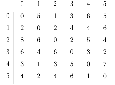
Table 2:The shortest-paths matrix for the graph in Figure 1