While dynamic programming can be successfully applied to a variety of optimization problems, many times the problem has an even more straightforward solution by using a greedy approach. This approach reduces solving multiple subproblems to find the optimal to simply solving one greedy one. Implementation of greedy algorithms is usually more straighforward and more efficient, but proving a greedy strategy produces optimal results requires additional work.

Activity Selection

Problem

Given a set of activities A of length n

S = <a₁, a₂, …, a_n>

with starting times

<s₁, s₂, …, s_n>

and finishing times

<f₁, f₂, …, f_n>

such that 0 ≤ s_i < f_i < ∞, we define two activities a_i and a_j to be compatible if

f_i ≤ s_j or f_j ≤ s_i

i.e. one activity ends before the other begins so they do not overlap.

Find a maximal set of compatible activies, e.g. scheduling the most activities in a lecture hall. Note that we want to find the maximum number of activities, not necessarily the maximum use of the resource.

Dynamic Programming Solution

Step 1: Characterize optimality

Without loss of generality, we will assume that the a’s are sorted in non-decreasing order of finishing times, i.e. f₁ ≤ f₂ ≤ … ≤ f_n.

Furthermore, we can define boundary activities a₀ such that f₀ = 0, and a_n+1 such that s_n+1 = f_n.

Define the set S_ij

S_ij = {a_k ∈ S : f_i ≤ s_k < f_k ≤ s_j}

as the subset of activities that can occur between the completion of a_i (f_i) and the start of a_j (s_j). Clearly then S = S_0,n+1, i.e. all the activities fit between the boundary activities a₀ and a_n+1.

Furthermore let A_ij be the maximal set of activities for S_ij, thus we wish to find A_0,n+1 such that |A_0,n+1| is maximized.

Step 2: Define the recursive solution (top-down)

Similar to rod cutting, if A_0,(n+1) ≠ ∅, then assume it contains activity a_k which will divide the set of activities into ones that all finish before s_k and ones that all start after f_k. Thus we can write the recursion as

and letting c[0,n+1] be |A_0,n+1|, i.e. c is the maximal number of compatible activities that start after a₀ and end before a_n+1, we can write the previous recursion as

i.e. compute c[0,n+1] for each k = 1, …, n and select the max.

We can show optimal substructure using a “cut-and-paste” argument by assuming that if c[0,n+1] is optimal, then c[0,k] and c[k,n+1] must also be optimal (otherwise if we could find subsets with more activities that were still compatible with a_k then it would contradict the assumption that c[0,n+1] was optimal).

Step 3: Compute the maximal set size (bottom-up)

Substituting i for 0 and j for n+1 gives

Note that S_ij = ∅ for i ≥ j since otherwise f_i ≤ s_j < f_j ⇒ f_i < f_j which is a contradiction for i ≥ j by the assumption that the activities are in sorted order. Thus c[i,j] = 0 for i ≥ j.

Hence, construct an n+2 x n+2 table (which is upper triangular) that can be done in polynomial time since clearly for each c[i,j] we will examine no more than n subproblems giving an upper bound on the worst case of O(n³).

BUT WE DON’T NEED TO DO ALL THAT WORK! Instead at each step we could simply select (greedily) the activity that finishes first and is compatible with the previous activities. Intuitively this choice leaves the most time for other future activities.

Greedy Algorithm Solution

To use the greedy approach, we must prove that the greedy choice produces an optimal solution (although not necessarily the only solution).

Consider any non-empty subproblem S_ij with activity a_m having the earliest finishing time, i.e.

f_min = min{f_k : a_k ∈ S_ij}

then the following two conditions must hold

1. a_m is used in an optimal subset of S_ij
2. S_im = ∅ leaving S_mj as the only subproblem

meaning that the greedy solution produces an optimal solution.

Proof

1. Let A_ij be an optimal solution for S_ij and a_k be the first activity in A_ij

   → If a_k = a_m then the condition holds.

   → If a_k ≠ a_m then construct A_ij^’ = A_ij - {a_k} ∪ {a_m}. Since f_m ≤ f_k ⇒ A_ij^’ is still optimal.

2. If S_im is non-empty ⇒ a_k with

   f_i ≤ s_k < f_k ≤ s_m< f_m

   ⇒ f_k < f_m which contradicts the assumption that f_m is the minimum finishing time. Thus S_im = ∅.

Thus instead of having 2 subproblems each with n-j-1 choices per problem, we have reduced it to 1 subproblem with 1 choice.

Algorithm

Always start by choosing the first activity (since it finishes first), then repeatedly choose the next compatible activity until none remain. The algorithm can be implemented either recursively or iteratively in O(n) time (assuming the activities are sorted by finishing times) since each activity is examined only once.

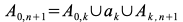
Example

Consider the following set of activities represented graphically in non-decreasing order of finishing times

Using the greedy strategy an optimal solution is {1, 4, 8, 11}. Note another optimal solution not produced by the greedy strategy is {2, 4, 8, 11}.

Greedy Algorithm Properties

A general procedure for creating a greedy algorithm is:

1. Determine the optimal substructure (like dynamic programming)
2. Derive a recursive solution (like dynamic programming)
3. For every recursion, show one of the optimal solutions is the greedy one.
4. Demonstrate that by selecting the greedy choice, all other subproblems are empty.
5. Develop a recursive/iterative implementation.

Usually we try to cast the problem such that we only need to consider one subproblem and that the greedy solution to the subproblem is optimal. Then the subproblem along with the greedy choice produces the optimal solution to the original problem.

Dynamic Programming vs. Greedy Algorithms

Often seemingly similar problems warrant the use of one or the other approach. For example consider the knapsack problem. Suppose a thief wishes to maximize the value of stolen goods subject to the limitation that whatever they take must fit into a fixed size knapsack (or subject to a maximum weight).

0-1 Problem

If there are n items with value v_i and weight w_i where the v_i’s and w_i’s are integers, find a subset of items with maximum total value for total weight ≤ W. This version requires dynamic programming to solve since taking the most valuable per pound item may not produce optimal results (if it precludes taking additional items).

Fractional Problem

Assume that fractions of items can be taken. This version can utilize a greedy algorithm where we simply take as much of the most valuable per pound items until the weight limit is reached.

---

---