Last lecture provided the framework for maximum flow problems and proved the key theorem - max-flow min-cut - that all algorithms are based on. This lecture we will investigate an algorithm for computing maximal flows known as Ford-Fulkerson.

Ford-Fulkerson Algorithm

The Ford-Fulkerson algorithm builds upon the general strategy presented last time.

	1.  for each edge (u,v) ∈ G.E
	2.     (u,v).f = 0
	3.  while there exists a path p from s to t in the residual network Gf
	4.     cf(p) = min{ cf(u,v) : (u,v) is in p}
	5.     for each edge (u,v) in p
	6.        if (u,v) ∈ E
	7.           (u,v).f = (u,v).f + cf(p)
	8.        else
	9.           (v,u).f = (v,u).f - cf(p)

This algorithm runs efficiently as long as the value of the maximal flow |f ^*| is reasonably small or if poor augmenting paths are avoided.

Edmonds-Karp Algorithm

An extension that improves upon the basic Ford-Fulkerson method is the Edmonds-Karp algorithm. This algorithm finds the augmenting path using BFS with all edges in the residual network being given a weight of 1. Thus BFS finds a shortest path (in terms of number of edges) to use as the augmenting path. With this modification, it can be shown that Edmonds-Karp runs in O(VE²).

Example

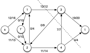
Consider the following flow network

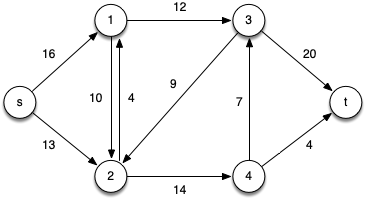
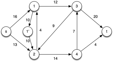
Initially we will remove the anti-parallel edges between vertices 1 and 2 by adding an intermediate vertex 1’ and edges with the same capacities, i.e. c(1,1’) = c(1’,2) = c(1,2) = 10.

Note that clearly |f ^*| ≤ 24 (the smaller of the capacities leaving the source or entering the sink).

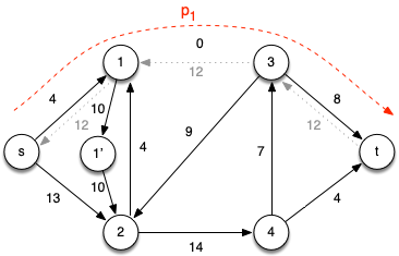
Iteration 1: Choose the augmenting path p₁ = < s, 1, 3, t > which has c_f(p₁) = 12 (due to c(1,3)) giving the residual network

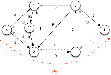
Iteration 2: Choose the augmenting path p₂ = < s, 2, 4, t > which has c_f(p₂) = 4 (due to c(4,t)) giving the residual network

Iteration 3: Choose the augmenting path p₃ = < s, 2, 4, 3, t > which has c_f(p₃) = 7 (due to c(4,3)) giving the residual network

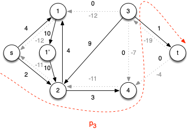
At this point there are no other augmenting paths (since vertex 3 is the only vertex with additional capacity to the sink but has no flow in from other vertices). Hence the final flow network with a min-cut shown is

with maximal flow |f ^*| = 19 + 4 = 23 (or 12 + 11 = 23).

Note As we admit flow along an edge (u,v), we create negative flow along the reverse edge (v,u), i.e. the flow provides capacity for that edge.

Consider the following example

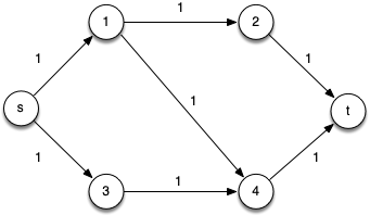
Clearly we can see that the max flow is |f ^*| = 2 since we could follow paths across the top (p₁ = < s, 1, 2, t >) and bottom (p₂ = < s, 3, 4, t >) of the graph.

Iteration 1: However, consider the following alternative initial augmenting path p₁ = < s, 1, 4, t > (which is valid since it also contains only 3 edges) which has c_f(p₁) = 1 giving the residual network

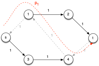
Notice that without the reverse edges, there is no augmenting path from s to t. However, because admitting flow produces capacity along the reversed edge (4, 1), the residual graph contains augmenting path p₂ = < s, 3, 4, 1, 2, t > which also has c_f(p₁) = 1 giving the residual network

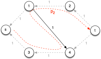
Note this second augmenting path essentially restores the capacity in the original edge (1, 4).

---

---