Single Source Shortest Paths - Dijkstra's Algorithm

Just as Prim’s algorithm improved on Kruskal’s algorithm for MST’s through the use of a priority queue, Dijkstra’s algorithm improves on Bellman-Ford for single source shortest path also through the use of a priority queue. Unlike Bellman-Ford, however, Dijkstra’s algorithm requires that all the weights are non-negative otherwise the algorithm may fail.

Dijkstra’s Algorithm

Dijkstra’s algorithm maintains a set S of vertices where minimum paths have been found and a priority queue Q of the remaining vertices under discovery ordered by increasing u.d’s.

DIJKSTRA(G,w,s)
1.  INITIALIZE-SINGLE-SOURCE(G,s)
2.  S = ∅
3.  Q = G.V
4.  while Q ≠ ∅
5.     u = EXTRACT-MIN(Q)
6.     S = S ∪ {u}
7.     for each vertex v ∈ G.Adj[u]
8.        RELAX(u,v,w)

INITIALIZE-SINGLE-SOURCE(G,s)
1.  for each vertex v ∈ G.V
2.     v.d = ∞
3.     v.pi = NIL
4.  s.d = 0

RELAX(u,v,w)
1.  if v.d > u.d + w(u,v)
2.     v.d = u.d + w(u,v)
3.     v.pi = u

Basically the algorithm works as follows:

1. Initialize d’s, π’s, set s.d = 0, set S = ∅, and Q = G.V (i.e. put all the vertices into the queue with the source vertex having the smallest distance)
2. While the queue is not empty, extract the minimum vertex (whose distance will be the shortest path distance at this point), add this vertex to S, and relax (using the same condition as Bellman-Ford) all the edges in the vertex’s adjacency list for vertices still in Q reprioritizing the queue if necessary

The run time of Dijkstra’s algorithm depends on how Q is implemented:

Simple array with search ⇒ O(V² + E) = O(V²)

Binary min-heap (if G is sparse) ⇒ O((V + E) lg V) = O(E lg V)

Fibonacci heap ⇒ O(V lg V + E)

Example

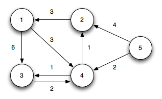
Using the same directed graph from chapter 21

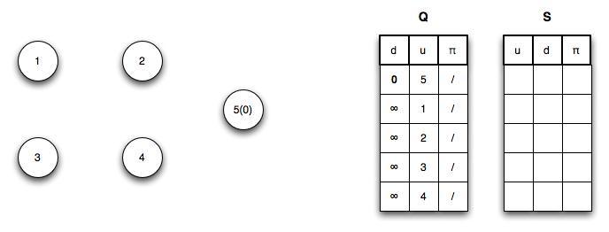
Using vertex 5 as the source (setting its distance to 0), we initialize all the other distances to ∞, set S = ∅, and place all the vertices in the queue (resolving ties by lowest vertex number)

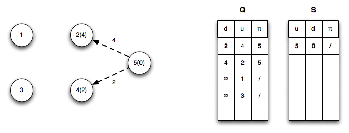
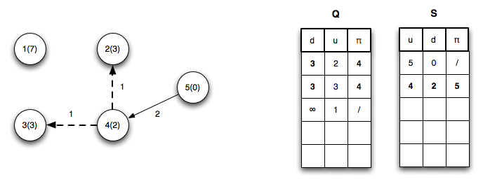
Iteration 1: Dequeue vertex 5 placing it in S (with a distance 0) and relaxing edges (u₅,u₂) and (u₅,u₄) then reprioritizing the queue

Iteration 2: Dequeue vertex 4 placing it in S (with a distance 2) and relaxing edges (u₄,u₂) and (u₄,u₃) then reprioritizing the queue. Note edge (u₄,u₂) finds a shorter path to vertex 2 by going through vertex 4

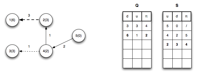
Iteration 3: Dequeue vertex 2 placing it in S (with a distance 3) and relaxing edge (u₂,u₁) then reprioritizing the queue.

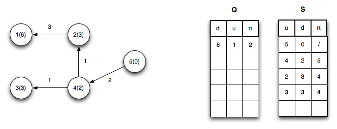
Iteration 4: Dequeue vertex 3 placing it in S (with a distance 3) and relaxing no edges then reprioritizing the queue.

Iteration 5: Dequeue vertex 1 placing it in S (with a distance 6) and relaxing no edges.

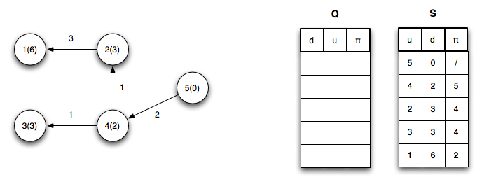
The final shortest paths from vertex 5 with corresponding distances is

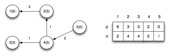
Just like Bellman-Ford, the path to any reachable vertex can be found by starting at the vertex and following the π’s back to the source. For example, starting at vertex 1, u₁.π = 2, u₂.π = 4, u₄.π = 5 ⇒ the shortest path to vertex 1 is {5,4,2,1}.