DFS can be used directly, but is more often used as an intermediate technique within another algorithm. This lecture examines three applications of DFS.

Parenthesis Theorem

DFS can be applied to parenthetical expressions by considering the final d’s and f’s by observing that for any u and v either

1. [u.d,u.f] and [v.d,v.f] are disjoint
2. [u.d,u.f] is entirely within [v.d,v.f]
3. [v.d,v.f] is entirely within [u.d,u.f]

If we view the depth-first tree from the example from chapter 17 as a timeline gives:

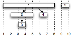
We can then substitute “(u” at each u.d and “u)” at each u.f such that the depth first tree (viewed as a timeline) represents a parenthetical expression. For example the final values above would represent the expression

( 1 ( 2 ( 33 ) 2 )( 44 ) 1 )( 55 )

Topological Sorting

A second application of DFS is to create a directed ordering of nodes, e.g. task dependencies. This can be done based on an important theorem that can be shown using DFS

A directed graph is acyclic (i.e. a DAG) if and only if a DFS produces no back edges.

Thus DFS can be used to test whether or not a graph has cycles on O(V+E) time.

Given a directed acyclic graph G (i.e. DAG, which can be determined via DFS), running DFS on G and sorting the vertices by decreasing finishing times produces a sequential ordering of the vertices. This can be seen since for any edge (u,v) in the depth-first tree, u must appear before v in the sorted list (since G is a DAG we know there are no back edges). For example, if the vertices represent a set of tasks with edges representing dependencies between tasks, a topological sort can be used to find a critical path. Since DFS runs in Θ(V + E), topological sort runs in the same time.

Strongly Connected Component Decomposition (SCCD)

The third useful application of DFS is to perform a strongly connected component decomposition. Given a directed graph G(V,E), the strongly connected component decomposition determines sets of vertices C_i ∈ V such that for every pair u,v ∈ C_i ⇒ u ↝ v and v ↝ u. In otherwords, it separates the graph into subsets of vertices that are mutually reachable from each other.

Define the transpose of a graph

i.e. it is the original graph with all edges reversed. The transpose graph can be created in O(V+E) time if the graph is represented as an adjacency list.

It can then be shown that u and v are mutually reachable from each other in G if and only if u and v are mutually reachable from each other in G^T.

Thus the procedure for finding strongly connected components is as follows:

1. Run DFS on G to find u.f’s ⇒ O(V+E)
2. Compute G^T ⇒ O(V+E)
3. Run DFS on G^T considering the vertices in decreasing order of u.f’s from step 1 ⇒ O(V+E)

The resulting depth-first trees from step 3 are the strongly connected components of G. Furthermore, the running time of SCCD is Θ(V+E).

Example

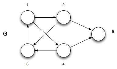
Consider the following directed graph

Step 1 - Run DFS on G

Running DFS on G (starting at vertex 1 and taking the vertices in numerical order) gives

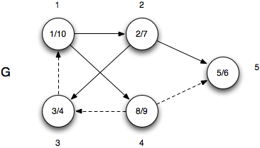
Thus the vertices in decreasing order of u.f is {1,4,2,5,3}.

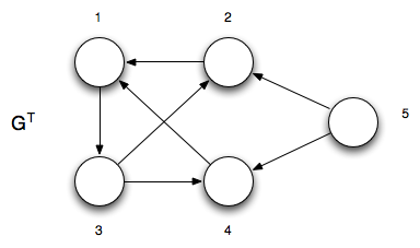
Step 2 - Compute G^T

The transpose G^T is

Step 3 - Run DFS on G^T

Running DFS on G^T taking the vertices in the order {1,4,2,5,3}

The depth-first trees from step 3 are

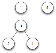
Hence the strongly connected components are {1,2,3,4} and {5}.

---

---