Related Books


Books / Analysis of Algorithms / Chapter 2
Insertion Sort
All sorting algorithms have the property that given a set of keys:
- Input: Sequence of numbers <a1,a2,…,an>
- Output: Permutation <a1‘,a2‘,…,an’> such that a1’ ≤ a2’ ≤ … ≤ an’
In this chapter
Insertion Sort Algorithm
Insertion Sort accomplishes this task by looping through each element moving it into place within the preceeding elements in the array. Thus insertion sort sorts in place, i.e. the array can be reordered with a constant (regardless of input size) amount of extra storage (in this case just a single temp variable for swapping). The pseudocode for the algorithm is:
INSERTION-SORT(A)
1  for j = 2 to A.length
2     key = A[j]
3     // Insert A[j] into the sorted sequence A[1..j-1]
4     i = j - 1
5     while i > 0 and A[i] > key
6        A[i+1] = A[i]
7        i = i - 1
8     A[i+1] = key
Proof of Correctness
In order to prove the correctness of an algorithm, i.e. that it will work for any input set, we construct a loop invariant which is a condition that holds for each iteration of the loop (thus the name invariant). Then the proof consists of verifying that the algorithm maintains the loop invariant for three conditions:
- Initialization - the loop invariant holds prior to the first iteration.
- Maintenance - if the loop invariant is true prior to an iteration, then it is still true after the iteration.
- Termination - the loop invariant is true when the loop terminates, i.e. after the last iteration thus producing the desired result
Note: This procedure is similar to an inductive proof with a base case and induction step but with an added termination criteria.
The loop invariant for insertion sort can be stated as follows:
At each step, A[1..j-1] contains the first j-1 elements in SORTED order.
The proof of correctness is then straightforward:
-
Initialization: Prior to the loop j =2 ⇒ A[1.. j-1] = A[1] which contains only the A[1.. j-1] elements (of which there is only one) and since there is only a single element they are trivially sorted.
-
Maintenance: The outer for loop selects element A[ j] and positions it properly into A[1.. j-1] via the while loop. Since the array A[1.. j-1] began sorted, inserting element A[j] into the proper place produces A[1.. j] in sorted order (and contains the first j elements).
-
Termination: The loop terminates when j= n+1 ⇒ A[1.. j-1] = A[1.. ( n+1)-1] = A[1.. n] which since the array remains sorted after each iteration gives A[1.. n] is sorted when the loop terminates (and contains all the original elements) ⇒ the entire original array is sorted.
Analysis
For all analysis in this course we assume that the algorithm will be implemented by a program run on a generic computer, i.e. single processor with random access memory (parallel algorithms are beyond the scope of this course but are extremely important in today’s computing environments).
We will define the input size, n, to typically be the number of elements in the input set (but it could represent the number of bits in a representation or other appropriate enumeration). The running time will then be the total number of execution steps as a function of n the algorithm takes to complete. We will assume that each line of pseudocode executes in a constant amount of time (although that amount may vary from line to line). Thus we multiply the (constant) time each line takes to execute by the number of times the line executes to find a cost per line and then sum the costs of all lines to give the run time of the algorithm.
For insertion sort we will define a variable tj to be the number of times the while loop test is performed (which will be one more time than the body of the loop is executed) where j =2,3,…, n with n = A.length.
General Run Time
The run time for insertion sort can then be written as

where the ci’s are the cost of each line (noting that c3 = 0 since line 3 is a comment).
Case 1: Best Case
The best case for insertion sort is when the input array is already sorted, in which case the while loop never executes (but the condition must be checked once). Thus tj = 1 for all j =2,3,… n (i.e. tj-1 = 0) and the run time reduces to:
which is a linear function of n.
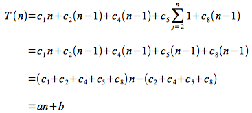
Case 2: Worst Case
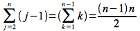
The worst case for insertion sort is when the input array is in reverse (decreasing) sorted order, in which case the while loop executes the maximum number of times. Thus tj = j for j =2,3,…, n. Using Appendix A of CLRS, the summation terms can be reduced as follows:
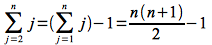
and
Thus the run time becomes

which is a quadratic function of n.
Usually we are only concerned with the worst case behavior for several reasons
- it gives an upper bound on the run time
- it occurs often for certain problems, e.g. searching for a non-existant element
- average case is usually close to the worst case, e.g. for insertion sort average case has tj = j/2 which still gives quadratic run time (only with different constants)
Asymptotic Analysis
As far as the run time dependency on n, the actual statement execution times are irrelevant, i.e. the ci’s can simply be lumped together. Furthermore as n becomes large (i.e. asymptotically), the highest order term will ultimately dominate the growth of the function (and is known as the measure of the order of growth). Finally we ignore the leading constant to give the asymptotic run time of insertion sort as Θ (n2).
Note: Asymptotic notation gives the rate of growth, i.e. performance, of the run time for large input sizes and is not a measure of the particular run time for a specific input size (which should be done empirically).