Related Books


Books / Analysis of Algorithms / Chapter 3
Empirical Analysis of Algorithm Runtime
In last chapter, we performed a detailed analysis of insertion sort only to end up discarding most of the work by only keeping the highest order term. We also discarded any constants to describe the asymptotic growth of a function based on the input size, i.e. for “sufficiently large” values of n. Often we would like to empirically measure the actual runtime of an algorithm as a function of input size to get an estimate of the constant for the highest order term as well as where “sufficiently large” behavior is exhibited.
Implementation
Our first step in benchmarking an algorithm is to implement the pseudocode in a programming language of our choice. The selected language should not affect the asymptotic behavior of the algorithm since the analysis is based on the pseudocode operation. The empirical behavior, however, can be affected by programming language and/or system used if our metric is “clock time”, i.e. the actual time it takes the algorithm to complete. Thus to make our measurements more consistent across systems, we will instead use a counter to simply count each execution of a line of pseudocode, i.e. essentially upper-bounding the execution time of any line of code by a constant. So as we implement the pseudocode, we simply increment a counter variable to accumulate the number of statements executed, ignoring the fact that one line of pseudocode may require several lines of actual code depending on the language used. Some general guidelines for properly counting are
- Function call statements DO NOT increment the counter since their runtime is evaluated by the execution of the function.
- Return statement DO NOT increment the counter.
- Loop statements, i.e. for and while, will execute one more time than the statements in the loop body. Hence a counter can be added both within and after the loop statement as follows
for (...) {
   count++;
   // Body of loop
}
count++;

while (...) {
   count++;
   // Body of loop
}
count++;
- For logical structures, i.e.if, if/else, if/else if/ else, there will need to be counters in each branch for the total number of conditions to ensure proper counting dependent on which branch executes. Note: if there is no else branch, one should be added with simply the count increment in the case when the condition is false to properly count the evaluation of the condition
if (...) {
   count++;
   // Body of if
} else {
   count++;
}

if (...) {
   count++;
   // Body of if branch
} else {
   count++;
   // Body of else branch
}

if (...) {
   count++;
   // Body of first if branch
} else if (...) {
   count += 2;
   // Body of second if branch
} else if (...) {
   count += 3;
   // Body of third if branch
} else {
   count += however many if conditions there are
   // Body of else branch
}
The following example shows the pseudocode for bubble sort and the corresponding C implementation with added counter increments
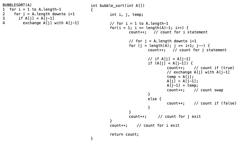
Note that even though the exchange takes three lines of C code, we only count the entire sequence once as it represents a single line of pseudocode.
Data Collection
Once the implementation is verified to be working, data can be generated for random inputs of various sizes and/or element ranges. For example, a table of output data for the bubble sort implementation where the first column represents the input size, i.e. number of elements in the input array, the second column is the average counts when run on arrays with elements in the range [1->32768], and the third column is the average counts when run on arrays with elements in the range [1->1024].
n Bubble-32768 Bubble-1024 16 341 337 32 1325 1312 64 5164 5092 128 20598 20513 256 81455 81858 512 328957 325107 1024 1311527 1313036 2048 5235204 5250859 4096 20961492 20923727 8192 83937509 83938403 16384 335295724 335134521 32768 1343230278 1339815632 65536 1068059893 1070383972
Graphical Evaluation
Plotting the data
Using a graphing program, e.g. spreadsheet, the data can be displayed graphically. Since these are empirical data points, they should appear on the graph only as points. Use a scatter plot such that n is the x axis and the runtime values are the y axis.
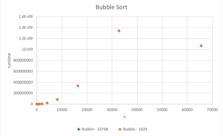
Note that for this example the two data sets are very close, thus the data points overlap. Furthermore, note that the last data point seems to be out of place with the other data. This may indicate an error in the code, or more likely in this case a numerical precision overflow. Thus this bad data point should be removed prior to fitting an asymptotic trend curve.
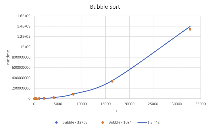
Adding a trend curve
Given that the asymptotic behavior for bubble sort is O(n2), we wish to fit a quadratic of the form cn2 to the empirical data points. However, since this asymptotic bound is only valid for sufficiently large input sizes, the curve should be biased to fit the larger input size data points more closely than the smaller input sizes. We will accomplish this by simply creating additional column(s) in our table that calculates the asymptotic values for a chosen value of c from the input size rather than attempt to use a regression curve fit. We can then add this column to the scatter plot displaying it as a curve rather than points and adjust c until the curve fits the larger points well.
n Bubble - 32768 Bubble - 1024 1.3 n^2 16 341 337 332.8 32 1325 1312 1331.2 64 5164 5092 5324.8 128 20598 20513 21299.2 256 81455 81858 85196.8 512 328957 325107 340787.2 1024 1311527 1313036 1363148.8 2048 5235204 5250859 5452595.2 4096 20961492 20923727 21810380.8 8192 83937509 83938403 87241523.2 16384 335295724 335134521 348966092.8 32768 1343230278 1339815632 1395864371